Difference between revisions of "Heterozygosity"
(→Infinite Alleles Model) |
(→Stepwise mutation model) |
||
| (17 intermediate revisions by the same user not shown) | |||
| Line 1: | Line 1: | ||
In population genetics heterozygosity is a measure of genetic diversity in a population. It represents an equilibrium between the input of genetic variation by mutation and the removal of variation by genetic drift. | In population genetics heterozygosity is a measure of genetic diversity in a population. It represents an equilibrium between the input of genetic variation by mutation and the removal of variation by genetic drift. | ||
| − | =Infinite | + | =Heterozygosity as an area= |
| + | |||
| + | [[File:Thetaarea.svg]] | ||
| + | |||
| + | One way to visualize heterozygosity (in terms of genetic diversity in a population) is as an area between 2''N'' and 2''μ''. Genetic variation is lost by drift at a rate of 1/(2''N''). So the inverse of this, 2''N'', can be though of as the amount of genetic variation that is retained in a population and not lost to drift. As described above mutations that are relevant to heterozygosity (average pairwise comparisons) are input into a population at a rate of 2''μ'' (where ''μ'' is the per generation mutation rate). The equilibrium level of genetic diversity as measured by heterozygosity is the product of the rate variation is added to a population and the amount of variation that can be maintained at any given time (think of this as almost like the size of a container, it can hold a certain amount before overflowing (or a funnel that drains slowly as new variants are added)); ''H'' = 2''N'' 2''μ'' = 4''Nμ'' = ''θ''. | ||
| + | |||
| + | Typically 2''μ'' will be a very small number and 2''N'' will be a very large number. Many orders of magnitude between these will cancel out as they are multiplied together. Also, you can see that a large population with a small mutation rate can have an equivalent level of genetic diversity as a small population with a high mutation rate. | ||
| + | |||
| + | =Infinite alleles model= | ||
| + | |||
| + | The image below represents three generations of a small population of six individuals per generation (''N''=6). Each individual is diploid and contains two copies of every gene in their genome (2''N''=12). Two gene copies are randomly sampled in the third generation and compared. There are two processes occurring each generation. Two lineages can come from the same copy in the generation before with a probability of 1/(2''N'') and therefore be identical to each other (and contribute to the overall rate of homozygosity in the population). Or a mutation could occur along one of the two lineages resulting in the gene copies being two different alleles from each other (and contribute to the overall rate of heterozygosity in the population). The probability of mutation is 2''μ'', where ''μ'' is the per generation per individual mutation rate; it is multiplied by two because a mutation could happen along either of the two lineages each generation resulting in the alleles being compared. | ||
[[File:Thetaderivation.svg]] | [[File:Thetaderivation.svg]] | ||
| − | + | These are two competing processes and the important factor is which process happened last in the history of the two gene copies. The top panel shows a mutation (represented by an *) occurring after a mutation; thus the two copies are heterozygous when compared. The lower panel shows coalescence of the lineages after mutation; thus the copies are homozygous. The total probability of both events per generation is 2''μ'' + 1/(2''N''). The probability the last event was a mutation as a fraction out of the total (and heterozygous in a direct pairwise comparison) is | |
| − | + | <math>H = \frac{2\mu}{2\mu + 1/(2N)}</math>. | |
| − | + | The rate of homozygosity is ''F'' = 1 - ''H'', which is | |
| − | + | <math>F = 1/(2N) / (2\mu + 1/(2N))</math>. | |
| − | + | We can rescale the terms in ''H'' by multiplying by 2''N''/2''N'' = 1. | |
| − | + | <math>H = \frac{2N}{2N}\frac{2\mu}{2\mu + 1/(2N)}=\frac{2N 2\mu}{ 2N 2\mu + 2N 1/(2N)} = \frac{4N\mu}{4N\mu + 1}</math>. | |
| − | + | ''θ'' is often used to represent 4''Nμ''. | |
| − | + | <math>H = \frac{\theta}{\theta + 1}</math>. | |
| − | + | This is the infinite alleles model, each mutation results in a new allele in the population. If ''θ'' is small relative to one then | |
| − | + | <math>H = \frac{\theta}{\theta + 1} \approx \frac{\theta}{1} = \theta = 4N\mu</math>. | |
| − | H | + | <math>H \approx 4Nμ</math>. |
| − | + | If ''θ'' is large relative to one then | |
| − | + | <math>H = \frac{\theta}{\theta + 1} \approx \frac{\theta}{\theta} = 1 = 4N\mu</math>. | |
| − | H | + | <math>H \approx 1</math>. |
| − | H | + | ''H'' increases approximately linearly with ''θ'' at small values but asymptotically approaches one (almost all pairwise comparisons are between different alleles) at higher values of ''θ''. |
| − | + | For example, [http://www.pnas.org/content/88/13/5897.short Hedrick ''et al''. 1991] found an average amino acid heterozygosity of approximately 6% at the MHC locus in humans. This implies that the rate of coalescence of two lineages is approximately 16 times larger (1/(16+1) ≈ 0.06) than the rate of amino acid altering mutations in the history of this gene. | |
| − | = | + | =Infinite sites model= |
| − | [[File: | + | [[File:Thetainfinitesites.svg]] |
| + | |||
| + | The probability of two ancestral lineages picking the same gene copy (coalescing) in the preceding generation is 1/(2''N''). The average amount of time until this takes is the inverse of the per generation probability or 2''N'' generations. Therefore, on average two lineages will coalesce 2''N'' generations in the past. If we track a DNA sequence that is inherited from a copy in the ancestor the two modern sequences will have an average of 4''N'' generations between them (2''N'' up to the ancestor and 2''N'' down to the other copy). These generations are multiplied by the per generation mutation rate ''μ''. A working assumption here is that each new mutation will change a different site or base pair along the DNA sequence (as if there were an infinite number of site to choose from). Therefore, the average nucleotide heterozygosity (the proportion of time two nucleotides are different in an alignment) within a population is ''H''<sub>n</sub> = 4''Nμ''. | ||
| + | |||
| + | In general per nucleotide mutation rates are very small and it is safe to assume that each new mutation within a population is likely to occur at a new basepair position. Two humans sequences will vary at about one out of 1,000 sites, which is lower than many eukaryotic species [https://www.ncbi.nlm.nih.gov/pmc/articles/PMC1204640/ Li and Sadler 1991]. However, there are exceptions. For example, [https://www.ncbi.nlm.nih.gov/pmc/articles/PMC4065115/ Cutter ''et al''. 2013] discus "hyperdiverse" species of nematodes, fruit flies, and tunicates that have levels of genetic diversity comparable to some bacterial and viral species. 10% of SNPs in ''Caenorhabditis brenneri'' are tri- or tetra-allelic. This violates assumptions of the infinite sites model and it has been suggested that more focus should be made on implementing finite site mutational models as a result. | ||
| + | |||
| + | [[File:Hyperdiverse.png|400px|Hyperdiverse species, Figure 1 of Cutter ''et al''. 2013]] | ||
| + | |||
| + | There are also examples of tri-alleleic SNPs in humans; these along with clusters of multiple mutations are found more often than expected (and the clustering is suggested to result from a form of polymerase error, [http://www.genetics.org/content/184/1/233 Hodgkinson and Eyre-Walker 2010]; [http://www.sciencedirect.com/science/article/pii/S0960982211005409 Schrider ''et a''l. 2011]; [http://genome.cshlp.org/content/24/9/1445.short Harris and Nielsen 2014]). | ||
| + | |||
| + | =Stepwise mutation model= | ||
| + | |||
| + | Some types of DNA sequences mutate more often by changing length rather than base pair substitutions. Microsatellites are a common example of this type of sequence among eukaryotic genomes. They are tandem repeats of a short nucleotide sequence. For example the following sequence contains a "CA" repeat. | ||
| + | |||
| + | CTACCTATGATGCACACACACACACACACACACACAATATCGCTAGAC | ||
| + | |||
| + | The CA repeats 12 times so we can represent the allele as (CA)<sub>12</sub>. An individual might be heterozygous with a (CA)<sub>8</sub> repeat at the same position on a homologous chromosome. | ||
| + | |||
| + | CTACCTATGATG'''CACACACACACACACACACACACA'''ATATCGCTAGAC | ||
| + | |||
| + | CTACCTATGATG'''CACACACACACACACA'''ATATCGCTAGAC | ||
| + | |||
| + | Microsatellites can have orders of magnitude higher mutation rates than nucleotide substitutions which means they are often highly variable and useful for some types of genetic studies (they can also be genotyped without sequencing). | ||
| + | |||
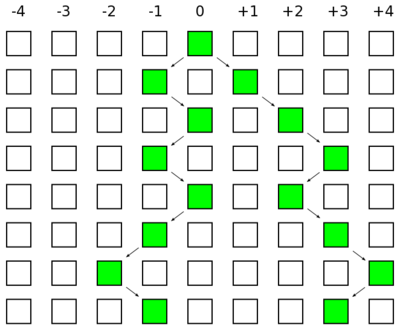
| + | [[File:1drandomwalk.svg|400px]] | ||
| − | + | A simple natural way to model microsatellite evolution is as a one-dimensional random walk. The figure above illustrates two simulated trajectories of a one dimensional random walk from a starting point at position zero. Many steps resulting in the final positions are obscured because of reversals of direction undoing the progress to the right or left. One property of these types of random walks is that the expected distance between the two walks is the square root of the total number of steps taken. A mutation is a change in length which corresponds to a step in this walk. | |
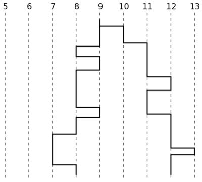
| − | + | The image above of a random walk might seem to imply that mutations happen at regularly spaced intervals. This is not the case; mutations are a stochastic process over time. The image below indicates what the trajectory of the allele repeats lengths might look like over time. | |
| − | + | [[File:Stepwisemicrosatellite.svg|400px]] | |
| − | + | On average we expect two lineages to have a common ancestor 2''N'' generations in the past (however, there is a large variance in this process). A pair of microsatellites are expected to, on average, have a total distance of 4''N'' generations between them with an expected 4''Nμ'' mutations between them (where ''μ'' is the per generation mutation rate). However, many of these mutations are obscured. Using the one-dimensional random walk model the best estimate of ''θ'' = 4''Nμ'' is the square of the difference in the length in repeat units between two alleles. | |
| − | + | In a large collection of alleles the variance (''σ''<sup>2</sup>) is the average squared difference from the mean, which is half of the average pairwise squared difference. Therefore, | |
| − | = | + | <math>\theta = 4N\mu = 2\sigma^2</math>. |
| − | + | [[Category:Population genetics]] | |
Latest revision as of 14:35, 20 October 2017
In population genetics heterozygosity is a measure of genetic diversity in a population. It represents an equilibrium between the input of genetic variation by mutation and the removal of variation by genetic drift.
Contents
Heterozygosity as an area
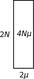
One way to visualize heterozygosity (in terms of genetic diversity in a population) is as an area between 2N and 2μ. Genetic variation is lost by drift at a rate of 1/(2N). So the inverse of this, 2N, can be though of as the amount of genetic variation that is retained in a population and not lost to drift. As described above mutations that are relevant to heterozygosity (average pairwise comparisons) are input into a population at a rate of 2μ (where μ is the per generation mutation rate). The equilibrium level of genetic diversity as measured by heterozygosity is the product of the rate variation is added to a population and the amount of variation that can be maintained at any given time (think of this as almost like the size of a container, it can hold a certain amount before overflowing (or a funnel that drains slowly as new variants are added)); H = 2N 2μ = 4Nμ = θ.
Typically 2μ will be a very small number and 2N will be a very large number. Many orders of magnitude between these will cancel out as they are multiplied together. Also, you can see that a large population with a small mutation rate can have an equivalent level of genetic diversity as a small population with a high mutation rate.
Infinite alleles model
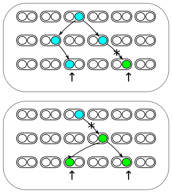
The image below represents three generations of a small population of six individuals per generation (N=6). Each individual is diploid and contains two copies of every gene in their genome (2N=12). Two gene copies are randomly sampled in the third generation and compared. There are two processes occurring each generation. Two lineages can come from the same copy in the generation before with a probability of 1/(2N) and therefore be identical to each other (and contribute to the overall rate of homozygosity in the population). Or a mutation could occur along one of the two lineages resulting in the gene copies being two different alleles from each other (and contribute to the overall rate of heterozygosity in the population). The probability of mutation is 2μ, where μ is the per generation per individual mutation rate; it is multiplied by two because a mutation could happen along either of the two lineages each generation resulting in the alleles being compared.
These are two competing processes and the important factor is which process happened last in the history of the two gene copies. The top panel shows a mutation (represented by an *) occurring after a mutation; thus the two copies are heterozygous when compared. The lower panel shows coalescence of the lineages after mutation; thus the copies are homozygous. The total probability of both events per generation is 2μ + 1/(2N). The probability the last event was a mutation as a fraction out of the total (and heterozygous in a direct pairwise comparison) is
[math]H = \frac{2\mu}{2\mu + 1/(2N)}[/math].
The rate of homozygosity is F = 1 - H, which is
[math]F = 1/(2N) / (2\mu + 1/(2N))[/math].
We can rescale the terms in H by multiplying by 2N/2N = 1.
[math]H = \frac{2N}{2N}\frac{2\mu}{2\mu + 1/(2N)}=\frac{2N 2\mu}{ 2N 2\mu + 2N 1/(2N)} = \frac{4N\mu}{4N\mu + 1}[/math].
θ is often used to represent 4Nμ.
[math]H = \frac{\theta}{\theta + 1}[/math].
This is the infinite alleles model, each mutation results in a new allele in the population. If θ is small relative to one then
[math]H = \frac{\theta}{\theta + 1} \approx \frac{\theta}{1} = \theta = 4N\mu[/math].
[math]H \approx 4Nμ[/math].
If θ is large relative to one then
[math]H = \frac{\theta}{\theta + 1} \approx \frac{\theta}{\theta} = 1 = 4N\mu[/math].
[math]H \approx 1[/math].
H increases approximately linearly with θ at small values but asymptotically approaches one (almost all pairwise comparisons are between different alleles) at higher values of θ.
For example, Hedrick et al. 1991 found an average amino acid heterozygosity of approximately 6% at the MHC locus in humans. This implies that the rate of coalescence of two lineages is approximately 16 times larger (1/(16+1) ≈ 0.06) than the rate of amino acid altering mutations in the history of this gene.
Infinite sites model
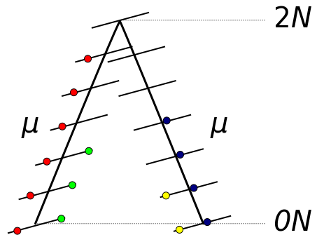
The probability of two ancestral lineages picking the same gene copy (coalescing) in the preceding generation is 1/(2N). The average amount of time until this takes is the inverse of the per generation probability or 2N generations. Therefore, on average two lineages will coalesce 2N generations in the past. If we track a DNA sequence that is inherited from a copy in the ancestor the two modern sequences will have an average of 4N generations between them (2N up to the ancestor and 2N down to the other copy). These generations are multiplied by the per generation mutation rate μ. A working assumption here is that each new mutation will change a different site or base pair along the DNA sequence (as if there were an infinite number of site to choose from). Therefore, the average nucleotide heterozygosity (the proportion of time two nucleotides are different in an alignment) within a population is Hn = 4Nμ.
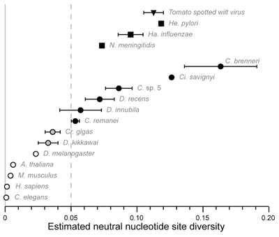
In general per nucleotide mutation rates are very small and it is safe to assume that each new mutation within a population is likely to occur at a new basepair position. Two humans sequences will vary at about one out of 1,000 sites, which is lower than many eukaryotic species Li and Sadler 1991. However, there are exceptions. For example, Cutter et al. 2013 discus "hyperdiverse" species of nematodes, fruit flies, and tunicates that have levels of genetic diversity comparable to some bacterial and viral species. 10% of SNPs in Caenorhabditis brenneri are tri- or tetra-allelic. This violates assumptions of the infinite sites model and it has been suggested that more focus should be made on implementing finite site mutational models as a result.
There are also examples of tri-alleleic SNPs in humans; these along with clusters of multiple mutations are found more often than expected (and the clustering is suggested to result from a form of polymerase error, Hodgkinson and Eyre-Walker 2010; Schrider et al. 2011; Harris and Nielsen 2014).
Stepwise mutation model
Some types of DNA sequences mutate more often by changing length rather than base pair substitutions. Microsatellites are a common example of this type of sequence among eukaryotic genomes. They are tandem repeats of a short nucleotide sequence. For example the following sequence contains a "CA" repeat.
CTACCTATGATGCACACACACACACACACACACACAATATCGCTAGAC
The CA repeats 12 times so we can represent the allele as (CA)12. An individual might be heterozygous with a (CA)8 repeat at the same position on a homologous chromosome.
CTACCTATGATGCACACACACACACACACACACACAATATCGCTAGAC
CTACCTATGATGCACACACACACACACAATATCGCTAGAC
Microsatellites can have orders of magnitude higher mutation rates than nucleotide substitutions which means they are often highly variable and useful for some types of genetic studies (they can also be genotyped without sequencing).
A simple natural way to model microsatellite evolution is as a one-dimensional random walk. The figure above illustrates two simulated trajectories of a one dimensional random walk from a starting point at position zero. Many steps resulting in the final positions are obscured because of reversals of direction undoing the progress to the right or left. One property of these types of random walks is that the expected distance between the two walks is the square root of the total number of steps taken. A mutation is a change in length which corresponds to a step in this walk.
The image above of a random walk might seem to imply that mutations happen at regularly spaced intervals. This is not the case; mutations are a stochastic process over time. The image below indicates what the trajectory of the allele repeats lengths might look like over time.
On average we expect two lineages to have a common ancestor 2N generations in the past (however, there is a large variance in this process). A pair of microsatellites are expected to, on average, have a total distance of 4N generations between them with an expected 4Nμ mutations between them (where μ is the per generation mutation rate). However, many of these mutations are obscured. Using the one-dimensional random walk model the best estimate of θ = 4Nμ is the square of the difference in the length in repeat units between two alleles.
In a large collection of alleles the variance (σ2) is the average squared difference from the mean, which is half of the average pairwise squared difference. Therefore,
[math]\theta = 4N\mu = 2\sigma^2[/math].
