Revision as of 22:45, 23 January 2016

Alleles are sampled from a population to make up the next generation. Anytime a random sample is taken it is likely to deviate slightly from the original population. Genetic drift is evolutionary sampling error. These deviations are not biased in any single direction towards an increase or decrease in frequency of a particular allele. However, these small deviations will accumulate over several generations and ultimately alleles will be lost until only a single allele remains in the population (assuming it is not reintroduced by mutation or from another population).

Basic Properties

The change in allele frequency due to genetic drift is without direction---it is just as likely to increase as to decrease---and is memory-less. Each generation is independent; the direction of frequency change in previous generations has no effect on the change in future generations.

The rate is change in allele frequency due to genetic drift is inversely proportional to the population size.

Complete loss (a frequency of zero) or fixation (a frequency of one) is an absorbing boundary. Once the allele frequency reaching this state it cannot return (due to genetic drift).

Ultimately an allele will reach loss or fixation within a population (if genetic drift is the only force acting).

The probability of ultimate fixation of an allele is its current allele frequency. The probability of loss is one minus the alleles current frequency. (All allele copies in the current generation have an equal chance of fixing, so the probability of a particular allele fixing is the number of copies it has out of the total.)

Variance

The variance in the change of allele frequency, p, between generations due to genetic drift is

[math]\sigma^2_p = \frac{p(1-p)}{2N}[/math]

This is derived from a binomial variance ([math]\sigma^2 = n p(1-p)[/math]) where the number of samples drawn from the population is [math]n = 2N[/math]. Since we are talking about an allele frequency between zero and one we rescale this variance by [math](2N)^2[/math] (the standard deviation, σ, is on a scale from zero to 2N) to put it on an interval from zero to one.

[math]\sigma^2_p = \frac{2N p(1-p)}{(2N)^2}[/math]

[math]\sigma^2_p = \frac{2N p(1-p)}{4 N^2}[/math]

[math]\sigma^2_p = \frac{p(1-p)}{2 N}[/math]

It is clear that genetic drift is strongest when the allele is at intermediate frequencies, p(1-p), and when the population size, N, is small.

The variance in allele frequencies between populations can be used as a way to define Effective Population Size, [math]N_e[/math].

Exact Binomial Probabilities

Genetic drift in a population can be represented as a transition matrix based on binomial probabilities. This equation gives the probability of going from i copies of an allele to j copies of an allele in a single generation.

[math]T_{i \to j} = {2N \choose j} \left( \frac{i}{2N} \right)^j \left( 1 - \frac{i}{2N} \right)^{2N-j}[/math]

For a tiny population of 2N = 4 this corresponds to:

[math]T_{i \to j} = \left( \begin{array}{ccccc} 1 & 0 & 0 & 0 & 0 \\ 0.316 & 0.422 & 0.211 & 0.047 & 0.004 \\ 0.062 & 0.25 & 0.375 & 0.25 & 0.062 \\ 0.004 & 0.047 & 0.211 & 0.422 & 0.316 \\ 0 & 0 & 0 & 0 & 1 \end{array} \right) [/math]

So, the probability of going from one copy of an allele to three copies of the allele in a single generation is 4.7%.

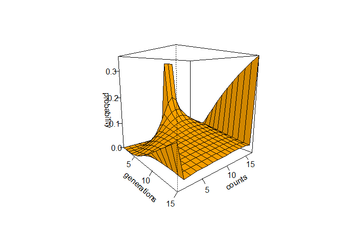
This can be iterated over several generations from a starting state to see how the probabilities of allele frequencies change. In the example below a starting frequency of 1/3 for 9, 10, and 11 allele copies in a population of 2N=16 is tracked over 15 generations.

Obviously, for large populations over many generations these calculations can get tedious.

Average Loss of Heterozygosity

If a small population becomes isolated so that there is no introduction of new alleles (for example in a captive breeding program or as a small number of founders on a new island) and genetic drift is a major force, the average loss of heterozygosity in the genome over multiple generations can be estimated.

[math]H_t = H_0 (1-\frac{1}{2N})^t[/math]

[math]H_t[/math] is the remaining heterozygosity at generation [math]t[/math].

[math]H_0[/math] is the initial heterozygosity at generation zero.

[math]t[/math] is the time in generations.

[math]N[/math] is the (diploid) population size.

The derivation of this stems from the probability of two allele copies being identical by descent over a period of time (and thus losing any potential starting difference between them). There are 2N total allele copies in the population. The probability of two alleles arising from the exact same copy in the previous generation is [math]1/2N[/math] (this is the rate of loss of variation per generation). The probability that this did not occur is [math]1 - 1/2N[/math] per generation. There is an independent chance of this each t generation so these probabilities are multiplied: [math](1 - 1/2N)^t[/math]. (If two randomly selected allele copies arose from the same copy in the previous generation then they cannot be heterozygous; thus, this is a way to keep track of the change in average heterozygosity in the population.) Wright formulated this as the rate of increase of identity-by-descent in terms of a "fixation" index F (variation is lost when a single allele reaches fxation, 100%, in the population). The increase in homozygosity (fixation) is one minus the decrease in heterozygosity. [math]F_t = 1-H_t[/math]. So, the amount of fixation over time t is [math]F_t = 1 - (1-\frac{1}{2N})^t[/math].

This can be simplified by using an exponential function approximation.

[math](1-\frac{1}{2N})^t \approx e^{- t/ 2N}[/math]

[math]H_t \approx H_0 e^{- t/ 2N}[/math]

The time until only half of the original genetic variation remains can be directly estimated as a rule-of-thumb.

[math]\frac{1}{2} = \frac{H_t}{H_0} \approx e^{- t/ 2N}[/math]

[math]\log{\frac{1}{2}} \approx \log{e^{- t/ 2N}}[/math]

[math]-0.6931 \approx - t/ 2N[/math]

[math]1.386 N \approx t [/math]

So, on average half of the genetic variation will be lost due to drift over a period of 1.386 N generations, where N is the diploid population size.

As an example, the 'alalā (Hawaiian crow, Corvus hawaiiensis) became extinct in the wild in 2002 and the species only exists as about 100 individuals maintained in captivity. This predicts that it will take 138 generations for the genetic variation (heterozygosity) of the species to decline by half (if the number of captive individuals remains constant each generation).

In another example, the resident human population of Pitcairn Island is about 50 individuals. If they became completely isolated from the rest of the world and maintained the same population size the majority of their current genetic variation is predicted to still be present in the population 2,000 years from now (assuming a generation time of 30 years).

Of course these examples assume an ideal random-mating population of constant size where each individual has an equal chance of reproducing. There are many ways this scenario can be altered to increase or decrease the rate of loss of genetic variation.

Simulation

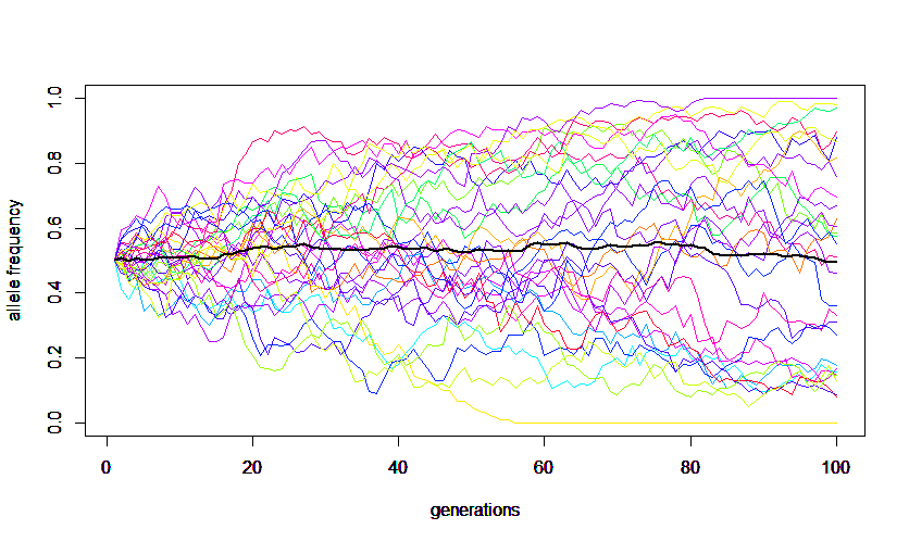
A forward simulation that keeps track of all allele copies in a population each generation is easy to understand but can run very slowly for large populations. The following code was used to make this image.

# a simple forward simulation of genetic drift in R

# start the timer
start <- proc.time()

# population size in number of organisms
N=100
# allele frequency
initp=0.5
# generations
gen=100
# number of replicant populations to plot
reps=10

# make an array of alleles to represent the population
pop<-list()
# population size in number of alleles
popsize=2*N
# make a list to record frequencies
freq<-list()

# uncomment to automatically clear last plot if any
# dev.off()

# list of random plotting colors
cl <- sample(rainbow(1000))

# loop through replicate lines to plot
for(r in 1:reps){
  
  # reset frequency
  p=initp

  # assign first generation of alleles
  for(i in 1:popsize){
    if(i<=p*popsize){
      pop[i]<-1
    }else{
      pop[i]<-0
   }
  }

  # loop through generations
  for(g in 1:gen){
  
    # calculate allele frequency
    sum=0
     for(i in 1:popsize){
       if(pop[i]==1){sum=sum+1}
    }
     p=sum/popsize
     print(paste(g,p))
    freq[g]<-p # record frequency
  
   # make a copy of the array
   pop.copy<-pop
  
   # randomly select values to replace
   for(i in 1:popsize){
     j=sample(1:popsize, 1)
     pop[i]=pop.copy[j]
    }
  
  }
  
  x<-c(1:gen)
  par(new=TRUE)
  plot(x,freq,type='l',ylim=c(0,1),col = cl[r],xlab="generations",ylab="allele frequency")
}

# show the run time
total.time<- proc.time() - start
print(total.time)

The R code below was used to generate the curve of allele frequency probabilities using a binomial transition matrix. It generated the following image:

# R code to generate Wright-Fisher probability plots of genetic drift
N=8 # diploid population size

n=2*N # number of gene copies

a=2*N + 1 # number of states from loss to fixation

g=15 # generations

# create an a-by-a matrix from an empty list
# have to tell it to treat as numbers with 'as.numeric()'
# or R will think they are characters and we can't
# do math operations on the cell entries
trans<-matrix(as.numeric(list()),nrow=a,ncol=a)

# create an a-by-g matrix for recording results
drifter<-matrix(as.numeric(list()),nrow=g,ncol=a)

# calculate binomial probability of each cell
for(j in 1:a){
  for(i in 1:a){
    trans[i,j]=dbinom(j-1, n, (i-1)/n)
  }
}

# look at result
# print(trans)

# vector of initial population states
vec=as.numeric(list(0,0,0,0,0,0,0,0,0,1/3,1/3,1/3,0,0,0,0,0)) # this needs to change if you increase pop size

for(i in 1:g){ # loop over generations
  
  drifter[i,]<-vec # use this if you want to plot the initial state
  
  # apply current state to the transitions
  nextgen<-vec*trans
  
  # print(nextgen)
  
  # need sum of columns for new state vector
  vec<-colSums(nextgen)
  
  #drifter[i,]<-vec # use this if you do not want to plot the initial state
  
}

print(drifter)

# make 3d plot with persp()
# http://stat.ethz.ch/R-manual/R-patched/library/graphics/html/persp.html
xposition = c(1:g) # labels for x axis tick marks
yposition = c(1:a) # labels for y axis tick marks
persp(xposition,
      yposition,
      drifter, # matrix of z values
      theta = 50, phi = 10, # adjust to rotate the view
      xlab = "generations", ylab = "counts", zlab = "probability", # axis labels
      shade=0.3, # adjust shading of surface
      ticktype="detailed", # show axis tick values
      col='orange',
      ltheta = 90, lphi = 45 # adjust the 'light' position
)

References and Footnotes