 ,
,Home > Science > Biology > Genetics > Population Genetics > Heterozygosity
Much of population genetics focusing on considering the expected relationship between pairs of genetic copies. Expected heterozygosity, or how frequently two copies of a locus are expected to differ, is an important theoretical concept, a natural way to quantify genetic diversity, and can be related to many other quantities of interest such as effective population sizes and migration rates. Expected heterozygosity is the opposite of homozygosity, how often genetic pairs are expected to be the same allele. It is important to realize that this is expected heterozygosity, if genetic copies in a population were randomly paired, not the actual fraction of individuals with heterozygous genotypes—in general we are not keeping track of individuals when thinking about heterozygosity, just allele frequencies in a population.
According to Hardy-Weinberg expectations for a locus with two alleles heterozygosity is expected to be
,where p is the allele frequency and H is heterozygosity (see Hardy 1908).
A more general equation for cases where there are more than two alleles is
or one minus the expected homozygosity. It is much easier to calculate the proportion of homozygotes, p2, then all of the possible combinations of heterozygotes (2pq+2pr+2qr+…), and just subtract them from one hundred percent.
Differences are created by mutations. When the transmission of two identical genetic copies (ones that are not already different and contribute to heterozygosity together) are considered from one generation to the next a mutation over either transmission results in a difference and contributes to heterozygosity.
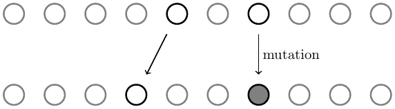
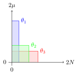
If μ is the per-generation mutation rate then the pairwise increase in heterozygosity is

(mutations between pairs that are already different do not increase heterozygosity, thus 1-H, and there are two transmission events that can possibly experience a mutation, thus 2μ).
Differences are lost by coalescent events. When a single genetic copy is sampled more than once in the next generation the new copies are identical to each other. If the total number of copies are held constant (2N for a diploid species (each individual has two copies of a genetic sequence), where N is the population size) then additional copies that are potentially different are lost when they are not sampled (coalescence of lineages back in time is genetic drift forward in time) and potential heterozygosity is lost.
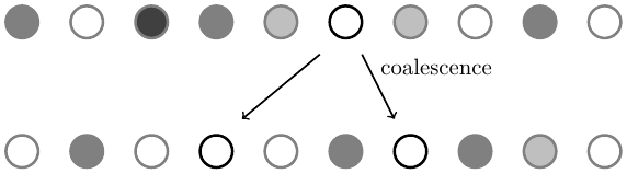
The probability of two copies originating from the same parental copy in the previous generation is
 .
.However, there are 2N possible parental copies in the previous generation so the per-generation rate of coalescence of two genetic copies is
 .
.Thus heterozygosity is lost at a rate of

(see Wright 1931).
At equilibrium the rate of input of genetic diversity is equal to the rate of removal.
 .
.This can be rearranged to
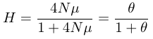 .
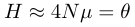
.θ = 4Nμ is a convenient shorthand in population genetics because 4Nμ, which represents a balance of mutation and drift, occurs quite often (different derivations and interpretations of θ will be described elsewhere).
This is an infinite alleles model, where each mutation results in a new allele yet the population size is finite and expected heterozygosity cannot be above 100%.
In the case where 4Nμ ≪ 1, which is often the case on the nucleotide level, 1 + 4Nμ ≈ 1 and
 .
.This is the infinite sites model, where each new mutation occurs at a new nucleotide site in a DNA sequence. In general this is a safe assumption for variation within a species but not between species unless they are very closely related.
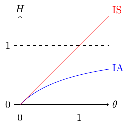
The figure above compares heterozygosity under the infinite alleles (IA) and infinite sites (IS) models. Infinite sites heterozygosity increases linearly with θ while infinite alleles approaches a limit at H = 1. However, in general the biologically relevant region is well within the area in the lower left corner where both models are essentially equivalent.
Average heterozygosity at a DNA sequence level can be used, along with an estimate of the mutation rate, to estimate the population size N.
Geraldes et al. (2008) found an average nucleotide heterozygosity of H = 0.00155 for the introns of four autosomal (not X or Y linked or mitochondrial) genes (Chrng, Med19, Prpf3, and Clcn6) in a sample of 60 house mice, Mus domesticus (or the subspecies Mus musculus domesticus) from Western Europe and Western Asia. (Table 2 of Geraldes et al. (2008) symbolized by π. θ represents a different estimate of 4Nμ in their table.) Geraldes et al. (2008) also estimate a per generation per nucleotide mutation rate of μ = 4.1 × 10⁻⁹ using divergence between species and estimates of the divergence and average generation times.
H = 4Nμ can be rearranged to N = H/(4μ). This gives N = 0.00155/(4 × 4.1 × 10-9) ≈ 95,000.
It is very hard to estimate actual numbers of house mice in the wild. However, ninety five thousand is clearly lower than what we expect. Of course there are a lot of assumptions at work here and if details like the average generation time change or the assumption of non-overlapping generations (overlapping generations experience a higher rate of drift, up to two times, which would double the N estimate) then the estimate will also change. However, population genetics is quite comfortable, as a general rule, with large amounts of uncertainty in estimates of parameter values, even if many of the underlying values are quantified precisely. This is also just a point estimate or expectation. The probability distribution of the range of likely values will be addressed elsewhere. A disconnect between actual and estimated population sizes introduces the concept of an effective population size (N versus Ne), which will also be addressed elsewhere.
In cases where a population has recently crashed to a much smaller population size the rapid loss of variation by genetic drift, ignoring the much slower input of new mutations, generates predictions of the loss of genetic diversity over time.
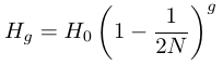
As described above the loss of heterozygosity (increase in homozygosity) each generation is expected to occur at a rate of 1/(2N). So the expected fraction of remaining heterozygosity is 1 - 1/(2N). Using g to indicate the generation
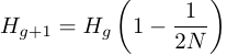 .
.It can quickly be seen that each additional generation involves multiplying by the expected remaining per-generation fraction of heterozygosity.

A continuous time approximation can be used to make the equation more mathematically convenient
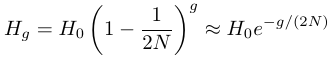 .
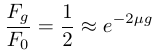
.This can be rearranged to solve for different relationships of interest such as
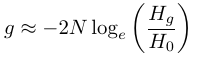
and
 .
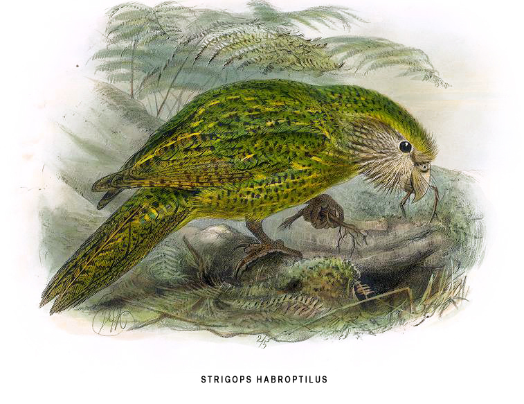
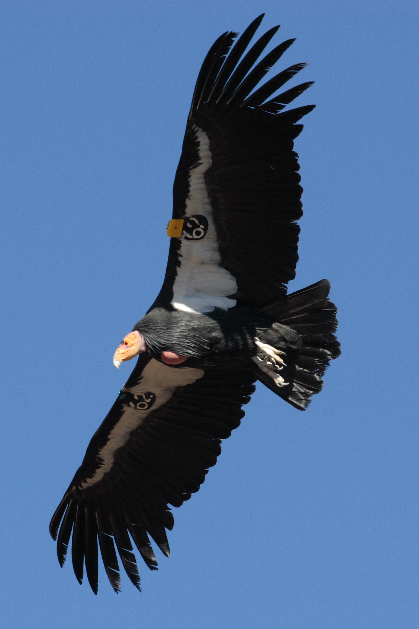
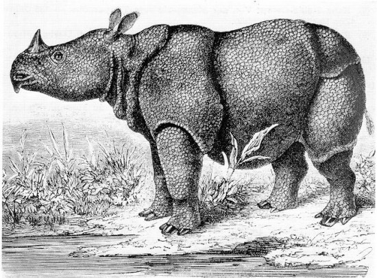
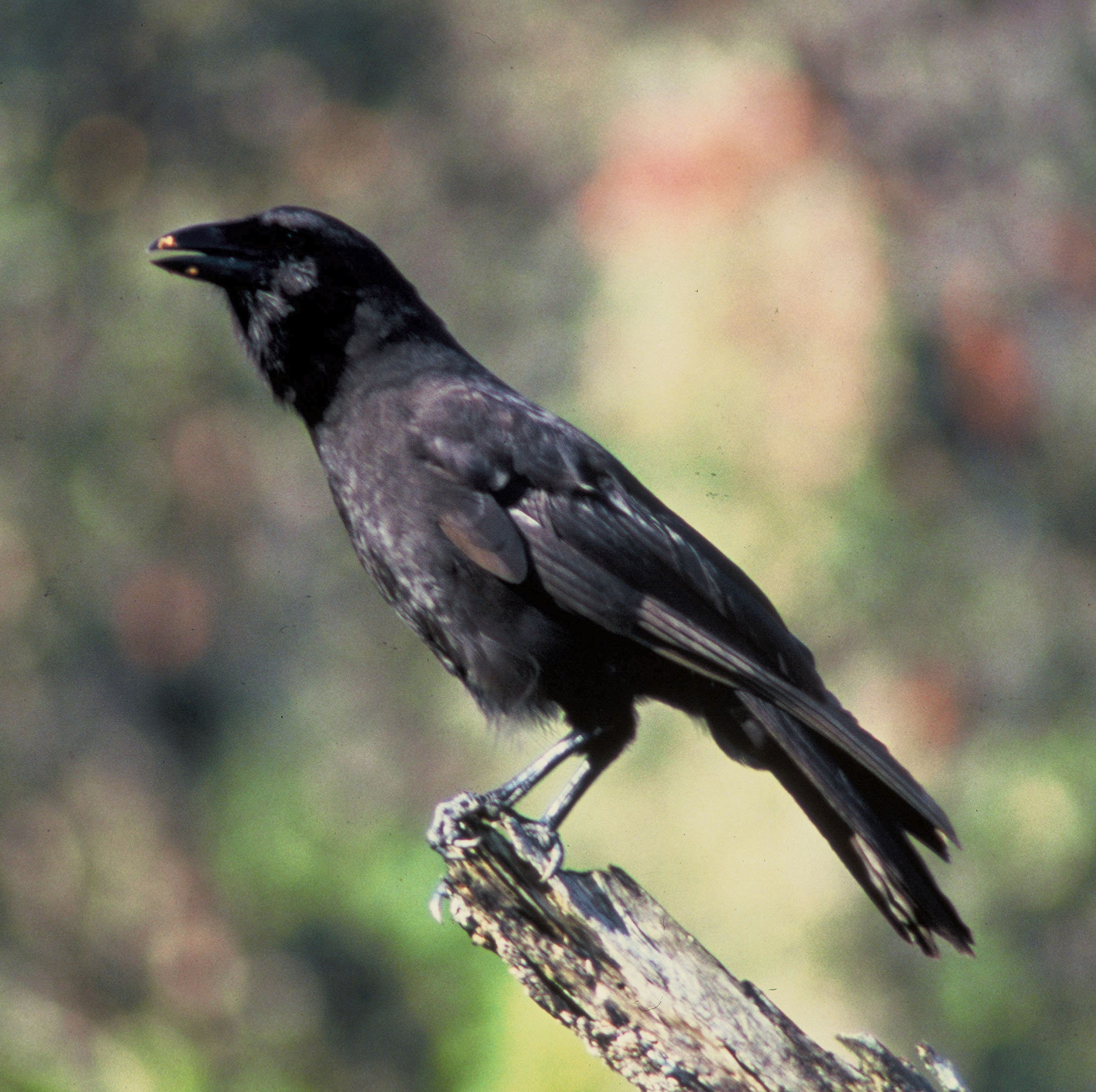
.Some species have severely reduced population sizes with a rapid predicted loss of genetic diversity due to drift. The kākāpō giant flightless parrot (Strigops habroptilus) of New Zealand reached a low of 51 individuals in 1995 (Powlesland et al. 2006), mainly because of introduced predators (e.g., cats, rats, and stoats). The ʻalalā (Corvus hawaiiensis) or Hawaiian crow became extinct in the wild in 2002 and is maintained at around 100 individuals in captive rearing (Tanimoto et al. 2017; Blanchet 2018). The California condor (Gymnogyps californianus) reached a low of 22 individuals in 1982 but now exists as a population of several hundred (Walters et al. 2010). There are only 62 individuals of the Javan rhinoceros (Rhinoceros sondaicus) in 2013 in a single population in Ujung Kulon National Park, Indonesia (Setiawan et al. 2017).
We can make predictions about the loss of genetic variation in populations of small numbers of individuals. For example, if a population is at a size of 75 individuals how long until 10% of its genetic diversity is lost?
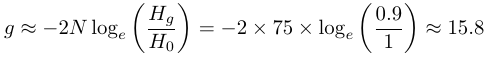
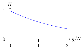
This 15.8 generations would be multiplied by the average generation time (from 25 to 30 years for the Javan rhinoceros and kākāpō to perhaps eight years for the ʻalalā). This assumes that each individual is equally likely to reproduce. If this is not the case then the time would be shorter. The plot below gives the expected decay in heterozygosity over N generations in an ideal population of constant size with equal probability of reproducing.
However, this assumes the population was much larger in the past and that the loss of genetic variation is presently the major force. Blanchet (2018) found that there was not a loss of genetic variation in the ʻalalā over time and that it has historically been at very low population numbers (i.e., near mutation-drift equilibrium).
Culver et al. (2008) compared the heterozygosities of endangered Florida panthers (Puma concolor couguar) from the 1980s to museum samples from the late 1800s to estimate the reduced population size in the wild.
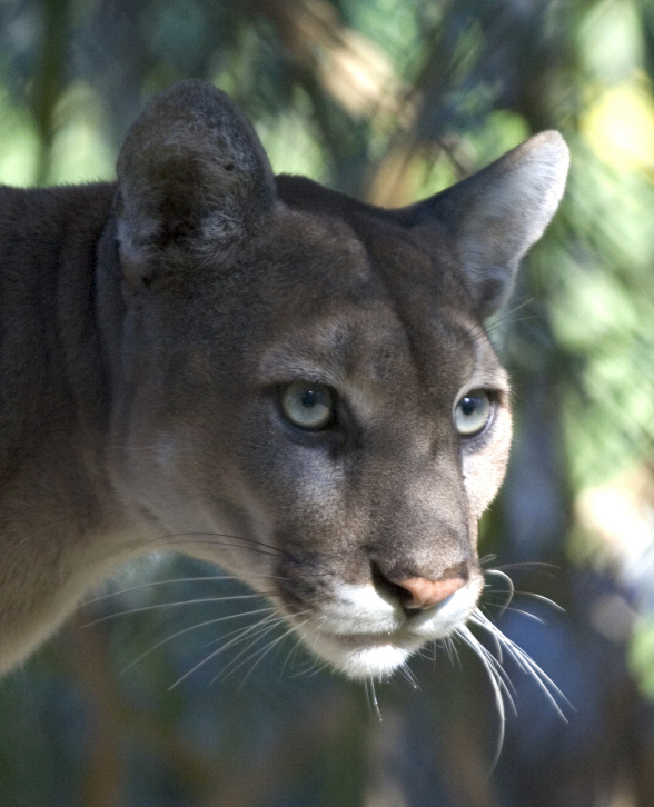
Using highly variable microsatellite loci they find an average heterozygosity of 0.311 in the ancestral population and 0.101 in the current sample of Florida panthers. (There is a small sample size correction used for an unbiased heterozygosity estimate that is not discussed here.) Assuming a generation time of five years and a time between the samples of 80 years gives 16 generations.
This 1/3 loss of heterozygosity works out to an effective population size of just over seven individuals. (Culver et al. 2008 finds a value of 7.4 instead of 7.11 and I am not sure where the error lies). They also consider stronger reductions for briefer periods of time and two deviations from an ideal population, unequal reproductive success and unequal male:female sex ratios. This is an extremely small population size and predicts a loss of 90% of genetic diversity in 32.7 generations or another 83.7 years if it remains at 7.11 individuals.
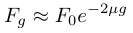
At the opposite end of a departure from equilibrium is a population that has dramatically increased in size so that genetic drift is minimized and diversity is increasing by new mutations. It is initially easier to look at this from the perspective of the change in homozygosity, F. From a pairwise comparison perspective homozygosity is broken by a mutation of either copy.
Using the same logic given above for the decay of heterozygosity we can quickly get
and
 .
.We can substitute in heterozygosity as one minus homozygosity and get the following.
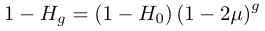
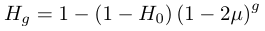
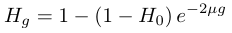
In order to illustrate the dynamics lets imagine genetic diversity has been strongly reduced by drift but the population has rebounded to a very large size (like an invasive species from a few founders or modern humans). Humans have a low level of genetic variation (a per nucleotide heterozygosity of approxiamtely 0.00088, Yu et al. 2003) and have recently expanded dramatically in population size to the billions. How long would it take for genetic diversity to double? To answer this to frame this in terms of how long until homozygosity is halved.
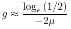
Using a per generation per nucleotide mutation rate of μ = 10-8, which is roughly on the order of the estimated human mutation rate (e.g., Rahbari et al. 2016 and references therein), gives 34.7 million generations. This is conservative, as the mutation-drift equilibrium point is approched the loss of diversity by drift becomes more important and it will take a longer time to regain diversity. The recovery of genetic variation by new mutations is extremely slow. For many species this is on a geologic timescale. Transient population crashes and accelerated drift can easily be a much stronger force than the increase in diversity by mutation. (However, some loci, such as microsatellites, have mutation rates several orders of magnitude higher than nucleotide substitutions and mutations over an entire gene region, such as those required to disrupt gene activity, are also higher and predict faster change due to mutation.)
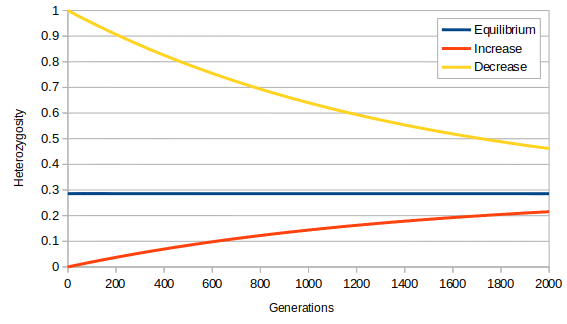
A very small population size, N = 1000, and high mutation rate, μ = 10-4, is used to illustrate the predicted change over time as heterozygosity approaches its predicted equilibrium value in the plot below.
Floyd A. Reed, December 4, 2020 – January 17, 2021