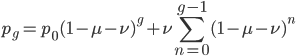
How do you permanently increase or decrease the fitness of a population (in terms of population genetics). Is it better to intensify the strength of selection so that deleterious mutations are removed, or relax the strength of selection so that mutations are better tolerated. This is something that is relevant to the current human condition, where there is an increased amount of medical intervention and (in the very recent past) a relaxation of some adaptive demands in the environment (this will be misunderstood, human culture has placed additional demands upon humans in the longer timescale, but anyway...). Arguments can be made for either scenario and---it turns out that it really doesn't matter. Strangely enough the strength of selection cannot change the average fitness (at equilibrium) of a population.
For this post only think of mutations as deleterious (they lower an organism's fitness) if they have any effect at all. Most mutations either have no fitness effect (are selectively neutral) or lower fitness. Very few mutations in the genome would actually increase the fitness of an organism (adaptive). Again think about making random changes to a car. Most changes, slightly reducing the length of the radio antenna, either make essentially no difference or, reroute the fuel line to the windshield wiper pump, are a very bad idea in terms of performance of the car. It would be very rare to make random changes that increase the performance of the car.
So, we know there are deleterious mutations that exist in a population that can result in what we identify in humans as a genetic disease. Many of these are recessive such as cystic fibrosis or Tay-Sachs disease; however, some are dominant such as Huntington's disease or Marfan's syndrome. And some do not fit this simple category such as X-linked hemophilia. Why do human and other species have so many deleterious alleles in the population?
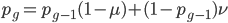
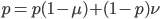
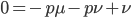
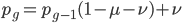
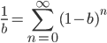
The alleles are generated by mutation and removed by selection. We can have a mutation rate  and a strength of selection (relative to unmutated alleles) acting on those mutations
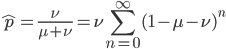
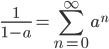
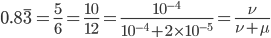
  . If we pretended the alleles acted independently, that pairing them together into diploid genotypes did not matter, then we can easily write down the equilibrium allele frequency,
  , of the mutation.

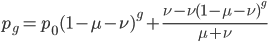
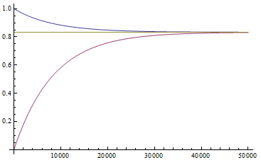
This is the rate that the allele is generated, , out of the total rate of input by mutation and removal by selection. For example, if the strength of selection against a mutant is 20% (a 20% fitness reduction relative to individuals with unmutated alleles) and the mutation rate is 0.1% then the equilibrium allele frequency is approximately one half of a percent, 0.5%. On the other hand if the fitness reduction is only 1% the allele can reach a higher frequency in the population at the same mutation rate (=0.1%) the equilibrium becomes approximately 9%, which is a dramatically high frequency for a dominant deleterious allele. (This is mathematically equivalent to bi-directional mutation; however, here the "back mutation" to restore the original state is selection.)
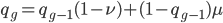
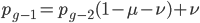
Now lets keep track of genotypes and the case where the fitness effect of the allele is dominant (with some simplifying assumptions). If it is dominant and deleterious it is probably rare (not like the 9% case above), so homozygotes,  are exceedingly rare and can be safely ignored because they contribute very little to the equilibrium dynamics. Mutations occur on the non-mutant allele copies
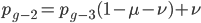
  (regardless if they are present in a homozygote or heterozygote). Selection removes a portion of heterozygotes, according to Hardy-Weinberg heterozygotes are expected to appear at a frequency of
  and an fraction of these are removed so the genotype rate of removal is
  .
.
( , the relative fitness to the unmutated homozygote is
  which adjusts the frequency of the heterozygotes due to selection.)
Only half of the alleles in the heterozygotes are the mutant allele so the rate of removal of the mutant allele is  . (Here we are focused on the case where the mutant allele is rare, which allows us to ignore
  in the first place. So,
  . The frequency of heterozygotes is then approximately
  . However, we want to keep track of the change in
  due to so we divide
  by 2. Selection is also removing non-mutant alleles in heterozygotes but the non-mutant homozygotes are much more common so we just ignore the other half of the alleles that are removed due to selection; this comes from the assumptions of large population size and rare mutant allele frequency.)
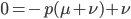
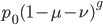
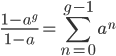
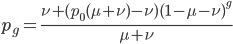
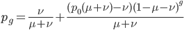
At equilibrium the rate of input and removal of the mutation are equal.
Rearrange and simplify.


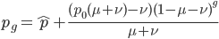
Using the two examples above with a mutation rate of  the equilibrium allele frequency is predicted to be 0.5% for a fitness reduction of 20% and 10% for a fitness reduction of 1%, which is almost equivalent to the case where alleles are acted on independently (as haploids). (If
  then
then  .)
.)
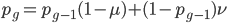
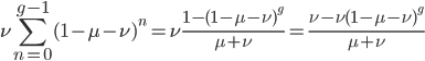
What if the fitness effect is recessive? Then selection only removes the mutant homozygotes which are predicted to occur at a frequency of . In this case selection can proceed more efficiently, in a sense, and mutant alleles are removed in pairs. All of the alleles in the homozygote are the mutant form so there is no adjustment necessary like dividing by two in the heterozygotes.
To keep this from getting messy let's use the trick now (which is actually less appropriate in this case because higher frequencies can be attained, but for now still assume that mutant alleles are very rare, , which is true for many mutations that result in human genetic diseases).


Using our two examples again, with a mutation rate of the equilibrium allele frequency is predicted to be 7% for a fitness reduction of 20% and 32% for a fitness reduction of 1%. Now the equilibrium allele frequencies are much higher, when very rare (when ) the difference can be many orders of magnitude. Masking the fitness effects in heterozygotes (carriers) allows the allele to get to unexpectedly high equilibrium frequencies.
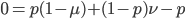
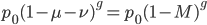
Now let's look at the average effect in the population. The average fitness  in a population can be calculated as the fitness of each genotype multiplied by its corresponding frequency. Let's say the fitness of unmutated homozygotes is 100% or 1. In the case of a dominant fitness effect

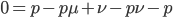
Expand and simplify
Let's say 

Substituting in 

The average fitness is one minus twice the mutation rate.
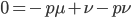
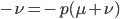
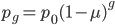
On the other hand if selection is recessive

Expand and simplify

Substituting in 

The average fitness is one minus the mutation rate.
Interestingly, the average fitness in the population does not depend on the fitness of the genotypes within the population; it is only a function of the mutation rate! (However, it does depend on the type of dominance; recessive deleterious effects result in both a higher equilibrium allele frequency and a higher average fitness.) This seems like a paradox at first. In our examples from above, if selection is dominant, then with a mutation rate of 0.1% the average fitness within the population is 99.8% regardless of how strong selection is against the mutation. If the mutation is recessive the average fitness is actually higher 99.9%, again regardless of the strength of selection against the mutation (this is related to selection being more efficient when it acts upon pairs of mutant alleles rather than one at a time in heterozygotes).
Why is average fitness only determined by the mutation rate? The trick to understand this is to realize that the strength of selection against a mutation and the frequency of the mutation in the population at equilibrium cancel out in terms of the average effect in the population. A mutation with a strong effect can only exist at a low frequency and only affect a few individuals, while a mutation with a weak effect attains a higher frequency and affects more individuals. The average effect of these two mutations, that have very different effects on fitness, in a population at equilibrium is the same.
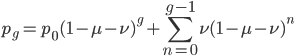
However, going back to the original question of this post, changing the mutation rate can permanently change the average fitness of a population. How do you change the mutation rate? Well certain chemicals and radiation are well known examples. (Also, in a recent article Michael Lynch points out that if relaxed selection affects mutations in genes that affect the mutation rate itself, DNA repair, etc., then there could be a feedback effect where selection does influence equilibrium average fitness by altering the mutation rate.)
To put this in perspective, mutations are not rare unusual events that can safely be ignored; they affect all of us. We all have new mutations that can be passed on to our children. Whole genome sequencing estimates this as high as to be around 40-80 new mutations depending on the age of our father. (Click on the image below for the source information.)
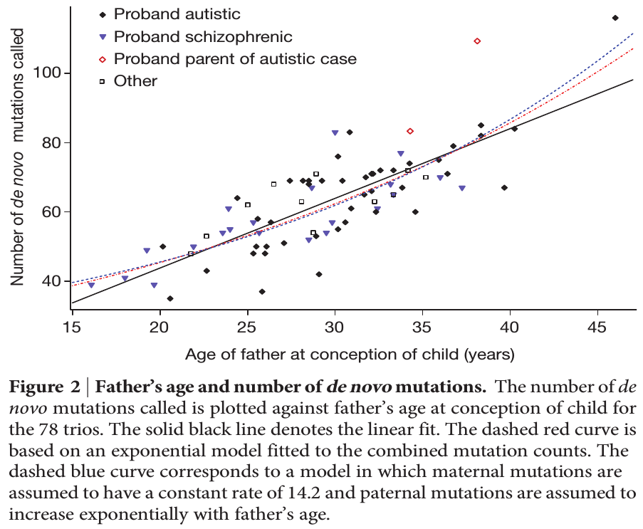
Each year of father's age adds on average two new mutations. The age of the father is also a risk factor for diseases like autism and schizophrenia and new mutations might be playing a role.
Above ground nuclear testing released large amounts of radioactive particles into Earth's atmosphere which spread planet-wide. At the height of the Cold War before the 1963 partial test ban the amount of radiation in the atmosphere was almost doubled (click on the image for a link to more information about how it was generated).

This had very real effects, for example it created a market for pre-war steel for specialized equipment like Geiger counters to test levels of radiation (steel made after WWII was contaminated with atmospheric radiation). A particularly valuable source are WWI battleship wrecks that are protected under water from contact with the atmosphere.
The increase in radiation alarmed some population geneticists like Hermann Muller who studied mutations and their effects on fitness. He helped raise awareness of the issue and his work among others contributed to the partial test ban treaty.
Furthermore, we come into contact with a wide range of industrial chemicals, many of which are seriously toxic and/or some of which can cause heritable mutations.
It is not known how this exposure might translate into increases in mutation rates (and to what degree this might contribute to the rates of genetic diseases). It would be interesting to estimate genome-wide mutation rates, in humans and other species if possible, over the last few centuries by comparing relatives sharing DNA sequences that are connected by different numbers of generations before and after certain points in history to see if there is a measurable effect.