A new collaborative publication is out in print: http://dx.doi.org/10.1111/jeb.13224

Abstract

A key component to understanding the evolutionary response to a changing climate is linking underlying genetic variation to phenotypic variation in stress response. Here, we use a genome-wide association approach (GWAS) to understand the genetic architecture of calcification rates under simulated climate stress. We take advantage of the genomic gradient across the blue mussel hybrid zone (Mytilus edulis and Mytilus trossulus) in the Gulf of Maine (GOM) to link genetic variation with variance in calcification rates in response to simulated climate change. Falling calcium carbonate saturation states are predicted to negatively impact many marine organisms that build calcium carbonate shells – like blue mussels. We sampled wild mussels and measured net calcification phenotypes after exposing mussels to a ‘climate change’ common garden, where we raised temperature by 3°C, decreased pH by 0.2 units and limited food supply by filtering out planktonic particles >5 μm, compared to ambient GOM conditions in the summer. This climate change exposure greatly increased phenotypic variation in net calcification rates compared to ambient conditions. We then used regression models to link the phenotypic variation with over 170 000 single nucleotide polymorphism loci (SNPs) generated by genotype by sequencing to identify genomic locations associated with calcification phenotype, and estimate heritability and architecture of the trait. We identified at least one of potentially 2–10 genomic regions responsible for 30% of the phenotypic variation in calcification rates that are potential targets of natural selection by climate change. Our simulations suggest a power of 13.7% with our study's average effective sample size of 118 individuals and rare alleles, but a power of >90% when effective sample size is 900.

My primary role was in running simulations and the power analysis of the genotype-phenotype associations. A few SNPs were found that were in significant association with calcification rates under stressful conditions. However, the power to detect these loci was low, less than 15%, which on the surface suggests that there are several more loci in the genome that also have an effect.

The discovered SNPs were also at very low frequency, which also suggests a slight ascertainment bias associated with their discovery (they happened to be included in the sample by chance compared to possible similar undiscovered rare SNPs that were not sampled). So, a way to correct for ascertainment bias was explored and incorporated into the power analysis.

Suppose the number of rare alleles included in a sample has a Poisson distribution with a mean of 1.13.

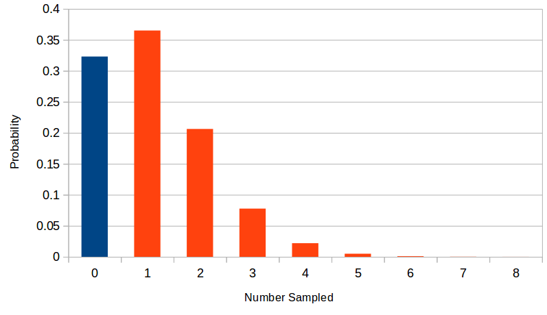
There is a significant part of the distribution at a sample of zero (in blue). We can only estimate allele frequency from the sampled alleles (in red). This shifts the weight of the distribution upward. In this example the sampled mean is 1.67 an increase of 47%.

We can work backwards to the underlying Poission mean from the observed counts by keeping track of the difference between the full Poisson distribution and the part above zero.

The distribution mean, , with ascertainment bias is related to the underlying mean, , by

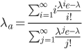
This is equal to

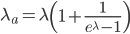
This is correct but it is in the wrong direction. We need to solve for . To do this we have to use the Lambert-W function, .

Honestly, this is not that useful because W cannot be expressed in terms of elementary functions but you can plug in values from a truncated Poisson distribution, numerically evaluate , and see that it works.

After correcting for ascertainment bias power can be evaluated with repeated simulations of multinomial draws for a given sample size and effect size.

In a 2x2 table of case controls and two different genotypes

genotype	AA	aa
case	a	b
control	c	d

The effect size can be quantified by

Evenly dividing the cases and controls, setting the corrected frequency out of 100 of 1.13, and an effect size of 10% gives the following cell probabilities.

genotype	AA	aa	total
case	0.4996	0.000365	0.5
control	0.4891	0.0109	0.5
total	0.9887	0.0113	1

These are used as multinomial probabilities and tested with a chi-square with a 1% cutoff in the following R script.

# sample size
n=600
# replicates
reps=100

sam <- numeric(length=100)
pow <- numeric(length=100) 
for(j in 1:100){
  n=j*100
  sam[j]=n
  q=power(n)
  pow[j]=q
  print(c(n,q))
}

power<-function(samplesize){
   count=0
   for(i in 1:1000){
      # generate multinomial random draw
      draw<-rmultinom(1, size = samplesize, prob = c(0.499635,0.489065,0.000365,0.010935))
      # save in 2X2 matrix form
      twobytwo<-matrix(draw, nrow=2, ncol=2)
      # run a chi square test
      result<-chisq.test(twobytwo)
      pval=result$p.value
      # extract p-value and record if below threshold
      if(is.na(pval)){pval=1}
      if(pval<0.01){count=count+1}
   }
   return(count/1000)
}

plot(sam, pow,log="x",type = "l", xlab="sample size", ylab="power")

This gives the following plot.

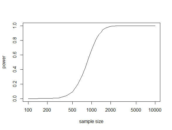
This shows a dramatic increase in power from a sample size of 600 to 1,200. Therefore, you would want to use an actual sample size of at least 1,000 under this scenario to have a reasonable chance of detecting a genotype-phenotype association of this size and frequency if it exists. If your sample size is below 400 (in this scenario) then you are just wasting time and resources.

The values and results above are just illustrative. In the blue mussel work the effect size was larger and tested in a different way. However, we found that we were at the lower edge of power in this kind of study (red circle over the solid blue line in the plot below).

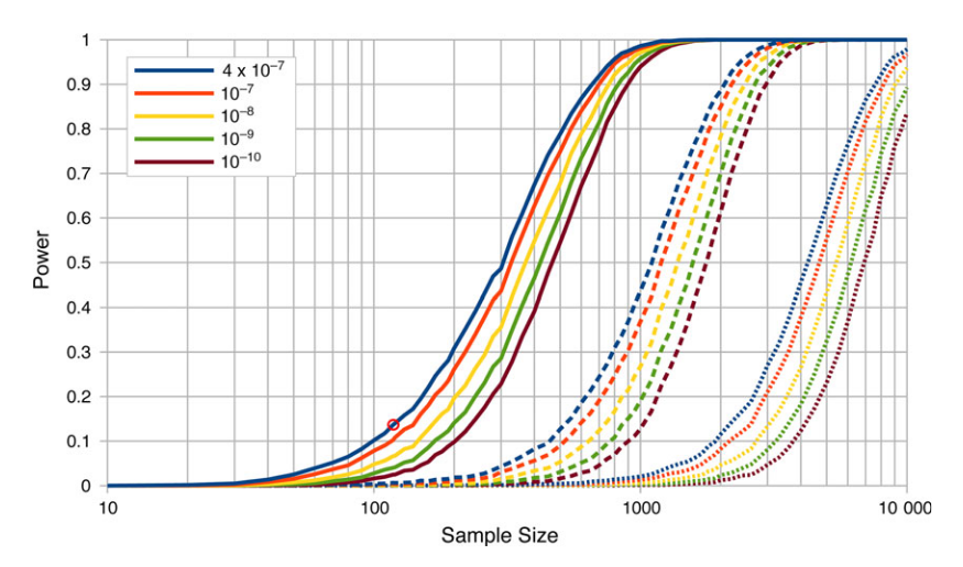
We had a power of only 14% and found three sites in significant association, which implies there are more to be found. The other colored lines show increasing significant cutoff stringency when correcting for multiple testing and the dashed lines are with the effect size halved and dotted line with the effect size quartered. If the study was done with a sample size of 1,000 all similar loci should be discovered and perhaps some of weaker effect.

There are a couple of other points to bring up related to this work. Briefly,

1. This was done in a zone of hybridization between two mussel species which increases the power to detect associations because of longer range linkage disequilibrium (and this comes along with some confounding issues).
2. Stressing the mussels exaggerates the phenotypic range, which, if there is underlying genetic variance influencing the phenotype, can uncover otherwise cryptic genetic influences on the trait being studied. In some ways this is similar to the often misunderstood phenomenon of genetic assimilation where altering the environment to exaggerate a phenotype can allow for more efficient selection to act upon otherwise subtle or completely hidden genetic influences upon a phenotype.
3. The variants associated with increased calcification under stressful conditions are at very low frequencies. If climate change results in strong selection for these variants it could still take centuries for them to increase to sufficient frequency to rescue mussel populations.