Lot's of different wave forms can be made by adding together harmonic series in certain ways.  A simple sine wave can have harmonics that vibrate twice as fast, three times as fast, etc.  Here is a plot of the odd numbered harmonics of a sine wave.

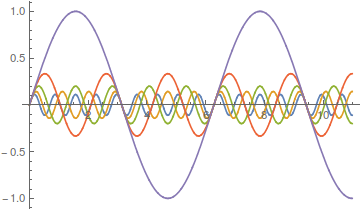
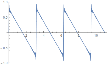
As the wavelength is reduced the amplitude of each wave is also purposely reduced.  It turns out that if you add these waves together you start approaching what is called a square wave.

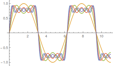
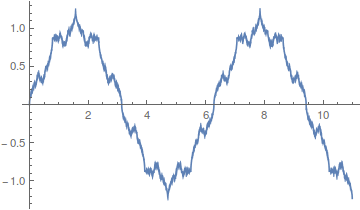
However, the approach can be slow.  There is a lot of wiggle in the waveform.  Below is a plot with 50 odd numbered harmonics added together; .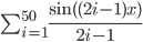

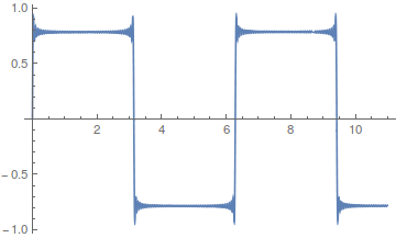
Closer, but you can still see the oscillation at the height of each peak.

If you add together the even harmonics, , you get a sawtooth wave.

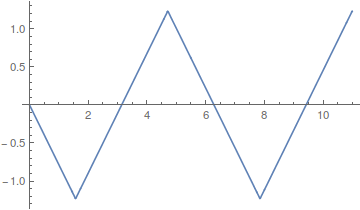
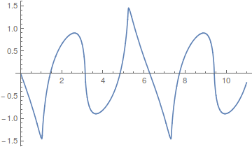
Odd harmonics with a different weighting scheme, 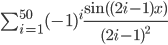, give triangular waves that converge quite fast.

Almost any waveform is possible, 

including this,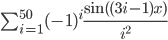 

Okay, so where am I going with this; there is a point here that ties back into population genetics.   Complex curves can be built up from the sum of a series of simpler curves.  However, it is also clear that in some cases the end result can take quite a large sum (the wiggle in the square and sawtooth waves above), in other words the final curve is slow to converge and requires a large number of harmonics.

Kimura's (1955) famous diffusion approximations to model the process of genetic drift in a finite population are built up in a similar fashion.  The final curve is a sum of an infinite series of higher order harmonics.  The math is messy.  It makes use of the hypergeometric function and Gegenbauer polynomials, but the underlying idea is similar to the examples given above.

In the simplest case of the diffusion approximation the series is

In this equation is the allele frequency, is the population size of diploid individuals, is the time in generations, which is often combined with in a parameter like , and is a hypergeometric function (specifically it is the ordinary Gaussian hypergeometric function ; there are many more but this is the most common).  In the graph below are the first six odd order curves of the series with and .

You can see that they tend to build (are positive) near the centre of the x-axis near a frequency of 0.5 and tend to alternative positive and negative near the edges cancelling each other out for a sum near zero.

Plotting these as sums of each new harmonic plus the previous ones gives these curves.

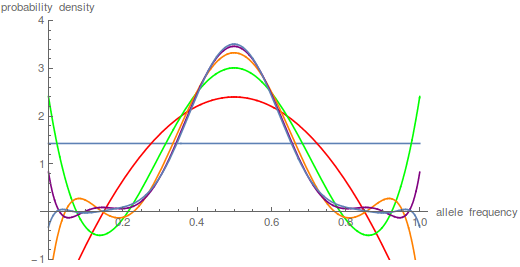
This plot just focuses on the last step, which is the sum up to in the equation.

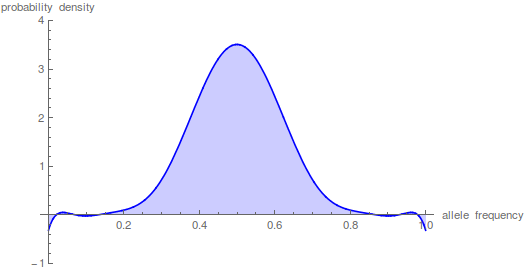
This is starting to give us the expected distribution of allele frequencies expected after N/10 generation of genetic drift when starting from a frequency of 1/2; however, the wiggle to positive and negative values near the edges means that it has not yet converged satisfactory.

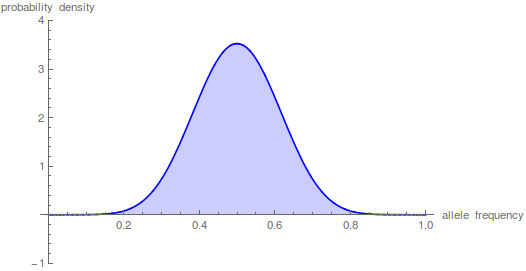
Taking the iterations up to gives a nice result.

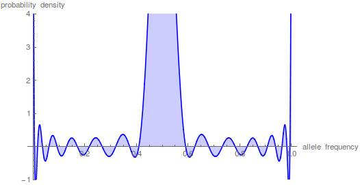
However, what if we want to look at even shorter periods of time.  Holding the y-axis scale the same and letting the peak run off the top of the graph look at what happens after just N/100 generations.

The sum has to be taken up to the to get things to smooth out.

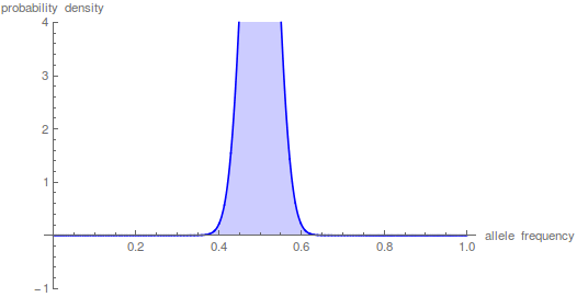
This takes some time on the computer---the hypergeometric function takes a bit of grinding to calculate.  Drift over shorter periods of time is precisely some of the situations where we might want to use this type of approach (it addresses standing variation and ignores new mutations that occur over deeper periods of time). This is why I have been exploring a faster alternative with the beta distribution that I wrote about in an earlier post.

By the way, I used mathematica to generate the plots above.  Here is the code if you are interested.

t = 10;
n = 1000;
p = 0.5;
m = 100;
(*the frequency distribution (probability) of the polymorphic \
fraction*)
poly =
Plot[Sum[p*(1 - p)*i*(i + 1)*(2*i + 1)*
Hypergeometric2F1[1 - i, i + 2, 2, x]*
Hypergeometric2F1[1 - i, i + 2, 2, p]*E^(-t*i*(i + 1)/(4*n)), {i,
1, m}], {x, 0, 1}, PlotRange -> {-1, 4}, Filling -> Axis,
PlotStyle -> Blue,
AxesLabel -> {"allele frequency", "probability density"}]

I also tried to plot this in R and got the following.

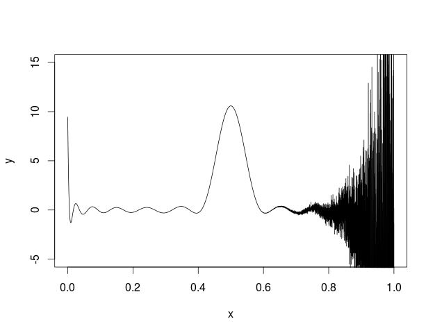
I'm not sure what is going on but some kind of error seems to be building across the function.

Here is my code
myDiffuse <- function(x,p,t,N,max){
max=25
sum=0
for(i in 1:max){
hypgeosumx=myHypergeoGaussSeries(i,x,max)
hypgeosump=myHypergeoGaussSeries(i,p,max)
sum=sum+p*(1-p)*i*(i+1)*(2*i+1)*hypgeosumx*hypgeosump*exp(-i*(i+1)*t/(4*N))
}
return(sum)
}

myKayAll <- function(i, l){
n=1
for(j in 1:(l-1)){
n=n*(j-i)*(j+1+i)
}
d=factorial(l)*factorial(l-1)
return(n/d)
}

myHypergeoGaussSeries <- function(i, z, m){
h=1
for(j in 2:m){
h=h+myKayAll(i,j)*z^(j-1)
}
return(h)
}

x <- seq(0, 1, len = 10001)
t=10
N=1000
p=0.5
max=5
y<-myDiffuse(x,p,t,N,max)

plot(x,y,type='l',ylim=c(-5, 15))