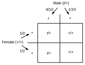
Here is an example of Bayesian statistics from genetics. Probabilities and frequencies have been rounded and some genetic details of the system are simplified for convenience; however, this should serve as a reasonable first pass approximation. The mouse t-haplotype is an example of meiotic drive (meiotic drive is a fascinating example of potentially powerful positive selection that does not necessarily result in Darwinian adaptation of the organism and in fact often lowers fitness). Heterozygote ($t$/+) males that have one copy of each allele, a $t$ allele and a wildtype “+” allele do not have an equal (1/2, 1/2) Mendelian probability of passing on each allele to their offspring. Rather there is a 90% chance of passing on the $t$ allele and a 10% chance of the “+” allele.
Incidentally $t$/$t$ homozygotes are immediately lethal and do not exist in the population.
The t-haplotype has an easily observable dominant phenotype. Heterozygous mice have much shorter tails than normal. In wild populations 5% of mice carry the $t$ allele (i.e., are $t$/+ heterozygotes).
You are doing a project on quantifying the reproductive success of male mice with the t-haplotype in the wild. However, you can only directly observe the offspring of individual (normal tailed, +/+) females without knowing the identity of the male parents. (Here assume each batch of offspring has only one male parent and belongs to the female it is found with in the nest.) You want to calculate the probability that the male parent was a $t$/+ heterozygote given the observation of the number of +/+ offspring. First off, before observing any more data, we can use the information of the 5% frequency of heterozygotes in the population from earlier studies. Our “prior” probability of a heterozygous father is $P(M_1) = 0.05$. Here were are using $P()$ to represent probability and $M_1$ to represent one of our models. A model is a hypothesis and our first hypothesis in this example is that the father is heterozygous. Our second model is that the father is a wildtype homozygote.
Let's say that we observe a single +/+ offspring. Now we need to calculate the probability of our data, $P(D)$. This is integrated over all models. Either the parent is a heterozygote, with a probability of 5% and the probability of a +/+ offspring is 10%, or the parent is a +/+ homozygote and the probability of a +/+ offspring is 100%. $$P(D) = 0.05 \times 0.1 + 0.95 \times 1 = 0.955$$ You can also see that $$P(D) = P(M_1) P(D|M_1) + P(M_2) P(D|M_2)\mbox{,}$$ where the | symbol means “given” so $P(D|M_1)$ is the probability of the data given model one is true. (In this case there are only two discrete models but we could integrate over more models or a range of parameter values for a model.)
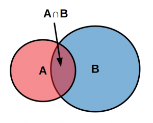
We are interested in the probability of the model given the data and it turns out that $$P(M) \cap P(D)=P(M|D) P(D) = P(D|M) P(M)\mbox{.}$$ The joint probability (intersection, $\cap$) of the model and the data is equal to both the probability of the model given the data times the probability of the data and the probability of the data given the model times the probability of the model—these are kind of flip side perspectives of looking at the same combinations of probabilities.
Perhaps it is a bit more clearer by looking abstractly at the intersection of A and B given that B happened. $$P(A|B)=\frac{P(A \cap B)}{P(B)} $$
The overlap of A and B out of the total B is the probability of A given B. This can be rearranged to $$P(A|B)P(B)=P(A \cap B)$$ and the same can be done for $$P(B|A)P(A)=P(A \cap B)\mbox{.}$$
For example, you go to a pet store looking for a small mammal with white fur. There is a box and you are told that one out of six animals in the box have white fur and that there are both eight mice and ten hamsters in the box for a total of 18 individuals. 2 of the mice have white fur and 1 of the hamsters have white fur. Before you reach in the box you know the probability of grabbing an individual with white fur is $3/18 = 0.1\bar{6}$ You reach in and can feel that you have grabbed a mouse but can't see it yet. Given that you have a mouse the probability of white fur is now $$P(\mbox{white}|\mbox{mouse})=\frac{P(\mbox{white}\cap\mbox{mouse})}{P(\mbox{mouse})}=\frac{2/18}{8/18}=1/4$$ and indeed 1/4 of the mice have white fur (2 out of 8). This is an awkward way to calculate the probability, but it does show the equation and relationship between the probabilities work.
Once we accept the relationships between the probabilities we can easily rearranged the system to the classical Bayesian equation $$P(M|D) P(D) = P(M) \cap P(D) = P(D|M) P(M)\mbox{,}$$ $$P(M|D) P(D) = P(D|M) P(M)\mbox{,}$$ $$P(M|D) = \frac{P(D|M) P(M)}{P(D)}\mbox{.}$$ The probability of the model (or hypothesis) given the data can be calculated from the probability of the data and a prior probability of the model.
Let's bring this into our example. $$P(M_1|D) = \frac{P(D|M_1) P(M_1)}{P(D)}\mbox{.}$$ We saw above that $P(D) = P(M_1) P(D|M_1) + P(M_2) P(D|M_2)\mbox{,}$ which makes this a bit more intuitive when we substitute it in. $$P(M_1|D) = \frac{P(D|M_1) P(M_1)}{ P(D|M_1) P(M_1) + P(D|M_2) P(M_2)}$$ The equation is really a fraction out of the total of all possibilities (of the data under all models). Even better, we have already worked out the values to plug in in order to do the calculation. $$P(M_1|D) = \frac{0.1 \times 0.05}{ 0.1 \times 0.05 + 1 \times 0.95} = \frac{0.005}{0.955} \approx 0.00524$$
This $P(M_1|D) \approx 0.00524$ is known as the posterior probability—the probability of our hypothesis after we have incorporated our prior and newly observed data. So, the observation of a single +/+ offspring brought the probability of a $t$/+ father down from 5% to approximately 1/2%. Congratulations, you are doing Bayesian statistics.
What if we observed a second +/+ offspring? The probability of the data under the first hypothesis is now $P(D|M_1) = 0.1^2=0.01$ and $P(D|M_2) = 1^2=1$. $$P(M_1|D) = \frac{0.01 \times 0.05}{ 0.01 \times 0.05 + 1 \times 0.95} = \frac{0.0005}{0.9505} \approx 0.000526$$ Alternatively, we could plug in our previous posterior, which already incorporates the first observation, into our prior for the next observation calculation (also realize that our new $P(M_2)' = 1-P(M_1)'$, where $P(M_1)'$ is the posterior from the first calculation). $$P(M_1|D) \approx \frac{0.1 \times 0.00524}{ 0.1 \times 0.00524 + 1 \times 0.99476} \approx \frac{0.000524}{0.995284} \approx 0.000526$$
However, if the third offspring has a short tail and is therefore a $t$/+ heterozygote then the probability under model two collapses. $$P(M_1|D) \approx \frac{0.1 \times 0.000526}{ 0.1 \times 0.000526 + 0 \times 0.999474} \approx \frac{0.000526}{0.000526} = 1$$ and $$P(M_2|D) = 1-P(M_1|D) = 0$$
Let's say that we didn't see a heterozygous offspring; how many observations are enough to be reasonably confident that the male parent was a +/+ homozygote? Bayes factor is a proposed way to address this. It is a ratio of the two probabilities of the data given the models (here $M_2$ is in the numerator because it has more support from the data). $$K = \frac{P(D|M_2)}{P(D|M_1)} $$ So with the observation of a single +/+ offspring $K_1 = \frac{1}{0.1} = 10$. Two +/+ offspring gives $K_2 = \frac{1}{0.01} = 100$. And we can quickly see that three +/+ offspring gives $K_3 = 1000$, etc. A $100>K>10$ is considered “strong” evidence of one hypothesis over the other and $K>100$ is considered “decisive” (Kass and Raftery 1995).
This is the tip of the iceberg. We can alter the models and inference in many ways. One common approach is to consider uncertainty in the strength of meiotic drive and/or its frequency in the population and estimate the distribution of the probability of these parameter values from the data (which in this case would be a set of offspring from multiple females) instead of assuming they are fixed values of 90% and 5% as is done here. Also, the number of parameters needed for more complex models can quickly increase in number, adding new dimensions with each parameter, and make calculations computationally expensive. Methods have been developed, such as Markov Chain Monte Carlo (MCMC) with the Metropolis–Hastings algorithm to efficiently explore the likelihood surface of high dimensional spaces. Finally, some probabilities are essentially impossible to calculate directly under a model but outcomes of the model can be easily simulated. This has lead to Approximate Bayesian Computation (ABC) approaches that estimate probabilities by brute force simulation.


