A year or two ago I wrote a letter of recommendation for grad school for a former student of my genetics class.  Last week they wrote me back and told me about their climate change manuscript (link) that was accepted for publication in Nature.  The publication was also picked up by the media.

Here is the message:

Cheers,"

It feels wonderful to get this kind of positive feedback from students from time to time.  In everyday teaching of a class it often feels like everyone is unhappy because you tend to only hear from the small fraction of students that complain.

Last Friday the lead author, Dr. Camilo Mora, gave a presentation on the work in our joint department seminar series.  Most climate change predictions focus on the dramatic increase in temperature in the polar regions--and indeed this is where the largest temperature changes are expected to occur.  But this is not the full picture.  One question is how long until we will experience unprecedented change that is outside the range of previous temperatures.  It turns out that this is predicted to happen first in the tropics, because the tropics have such stable temperatures, a smaller change can push the climate outside of the normal historical boundaries.  The problem is that tropical species and environments cannot handle temperature changes as well as temperate and polar species, because they have not had to adapt to wide swings of temperature in the past.  Another problem is that tropical countries tend to have less economic resources to deal with these changes.  The predictions for "climate departure" for some of the tropics are surprisingly near with some dates as soon as 2020.

Dr. Mora was able to do this as a student class project and with very little resources available, using a lot of free tools and data available online.

Here are some news links:

http://www.latimes.com/nation/la-sci-climate-change-tropics-20131010,0,482935.story

http://www.popsci.com/article/science/no-year-after-2047-will-be-cool-now

http://www.nytimes.com/2013/10/10/science/earth/by-2047-coldest-years-will-be-warmer-than-hottest-in-past.html?_r=0

http://articles.washingtonpost.com/2013-10-09/national/42849788_1_climate-change-intergovernmental-panel-global-ecology

http://www.natureworldnews.com/articles/4389/20131009/places-earth-experience-radically-different-climate-2047.htm

http://www.weather.com/news/climate/2047-coldest-years-may-be-warmer-hottest-past-20131009

http://www.cbc.ca/news/canada/north/world-temperatures-go-off-the-chart-by-2047-study-says-1.2053488

http://www.sciencedaily.com/releases/2013/10/131009133216.htm

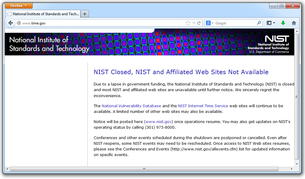
We had an exam yesterday in my genetics class.  During the exams I project the official time for Hawai'i on the screen so that my students can easily see how much time they have left.  However, because of the budget negotiation failure and partial government shutdown, the website I usually use was not available.  I projected it on the screen anyway.

And in the lower corner I opened the computer's clock settings so they could see that instead.  I announced that the government may be shutdown but we are not, so we are still having the exam today.  I also added that they may want to contact their representatives.

The idea that ancestral lineages come together (coalesce) at some point in the past is a powerful and useful concept in population genetics.  We inherit our copies of our genes from a finite number of ancestors.  If we randomly picked two copies of a gene in the population there is a chance each generation back that they are inherited from the same ancestral copy.

The number of copies of a gene in the population is twice the population size, or .  For example I have two "non-taster" alleles of the gene TAS2R38 and can not taste PTC.  These alleles are found all over the world.  If we look at the allele I inherited from my father, there is a chance that another random copy picked from the present human population is also inherited from the same copy from my father (by my brother or sister).  Moving further back in time my lineage intersects with my close cousins so that we inherited the same copy from our grandparents or great grandparents.  Even further are distant cousins with connections via more ancient common ancestors, and ultimately all modern humans and common ancestors hundreds of thousands of years ago.  Even the "taster" and "non-taster" allele branches are united in a common ancestor with some mutations along one lineage that converted a "taster" ancestor into a "non-taster" allele for people around the world to inherit.

On the simplest level, this probability of inheriting the same copy one generation ago is , or one out of the total number of possible gene copies to pick from (assuming the population size is a constant each generation).  Once ancestral lineages come together to the same copy they cannot "uncoalesce" and split back apart; so eventually all lines of inheritance will trace back to one common ancestor in the distant past.

This describes an exponential "waiting-time" process, like radioactive decay or the example I talked about earlier with non-reversible mutations; however, this looks back in time to when an event happened instead of the time until it will occur in the future.  In my class I often use flipping coins or rolling dice as examples to illustrate this.  The chance of rolling a "three" on a die is so on average you need six rolls to get a three.  The chance of "tails" from flipping a penny is .  You could get this on the first try, or it might take a few tries, on average it takes two coin flips.  This is a shared property of all exponential distributions (technically it is actually a geometric distribution because we are thinking of discrete generations, but with a large population we can assume a continuous time approximation and use the exponential).  The rate of coalescence of two lineages each generation is .  So, on average we wait a total of generations until the copies came from a common ancestor.  (The mean of an exponential distribution is the inverse of the rate parameter.)

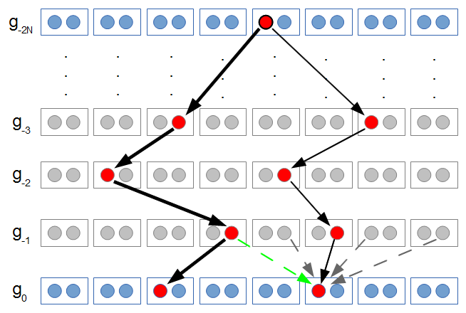
In the figure above copies of a gene are indicated by circles.  They are in pairs in each individual (rectangles).  I randomly pick two copies to compare in the current generation (red circles in the row).  The first copy on the left has a line of inheritance traced back to earlier generations by the thick black arrows.  There is a chance () that the second copy coalesces with the first in the previous generation (suggested by the green dashed arrow) but there is a much higher likelihood that it does not coalesce (, suggested by the gray dashed arrows).  In fact we expect coalescence to happen, on average, generations in the past.

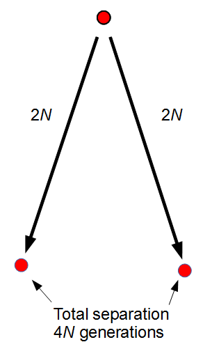
The total distance between two copies in the current generation is, starting from one, generations back to the common ancestor and down to the other copy.  This is a total distance of generations.

If we include a per generation mutation rate of to trace along this lineage with an average length of , we expect an average difference (or an average heterozygosity) in the population between two copies of a gene of (if each mutation affects a different nucleotide in the gene sequence so we see all of the events, which is generally expected for short time periods).  This measure of genetic diversity is a function of both the population size and the mutation rate .  Larger populations can accumulate more diversity before it is lost due to genetic drift and higher mutation rates introduce diversity at a greater rate.  This value of comes up frequently in population genetics and has its own symbol, .

For example, looking at the same thing in a different way.  The number of new mutations at a gene in a population each generation is .  There are copies of the gene in the diploid population and the fraction of them are expected to mutate each generation: .

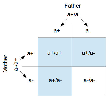
In my genetics class we start off with Punnett squares as a tool to generate the relative numbers of expected offspring from a cross.  In the simplest form we have two alleles at a single gene.  If there is a simple dominant/recessive phenotype pattern it can illustrate why we expect a three to one ratio of offspring phenotypes from a cross between two heterozgytoes (individuals that have two different types of alleles).

One of the nice things about working with yeast in the lab is that you can grow it as a haploid (only one copy of each gene) or as a diploid (two copies of each gene); the cells grow and divide in either form.  There are two mating types of cells, like male and female types in animals.  In yeast the mating types are MATa and MATα, or a and α (alpha) for short.  If cells of the two different mating types are growing near each other they will attempt to cross and create a diploid cell.

I used this as one of the introductory lab exercises in my genetics class.  We grew haploid wildtype (white colonies) and haploid mutant cells on a plate of media.  The mutants cannot produce adenine and are dark red because of oxidation of a precursor compound (in the adenine biosynthesis pathway) that accumulates in their cells.

I tried this out first and plated the mutant and wildtype haploid cells for each mating type a and α.  Then after these had grown overnight I spread the cells over each other in four spots corresponding to each cross.  Three of these diploid offspring cells turned (mostly) white, the dominant phenotype, and one was red because it had two mutant copies of the gene; illustrating the 3:1 phenotype ratio.

Above and below I've added genotype labels to try to illustrate.  Right and left are reversed but compare the image below to the Punnett square at the top of this post.

And below is a cross plate that one of the student groups (they work in groups of four in the lab) made.  It shows the heterozygotes being dominantly white colony phenotype even clearer than in my plate.