In an earlier post I went through a derivation of the Jukes Cantor model (based on a Poisson distribution of mutation events) and got the following type of relationship.
 ,
,
where  is the fraction of divergent sites between two DNA sequences and
  is the time the sequences diverged from a common ancestor in units of
  where
where  is the number of generations and
  is the per generation per nucleotide mutation rate.
This can be rearranged to

to convert an observed difference between two sequences into a corrected estimate of the divergence between two species.
However, this is only a point estimate and cannot handle cases where the fraction of sites that differ happen to be above 75% (this is possible by chance but becomes a log of a negative number and undefined).
We can rewrite this in a different way, as a binomial probability, and evaluate the probability of a data set over a range of divergence and place intervals around our point estimate.
As above, the probability that two nucleotides are different is
 .
.
Assuming each nucleotide is independent in a comparison of two sequences we can multiply by the number of sites that are different,  .
.

On the other hand two nucleotides can be in the same state if no mutations occurred, which is a probability of  (this comes from the Poisson distribution the model is based on, look back at the earlier post if this isn't clear) or mutations could have occurred along the lineages but they happened to end up as the same nucleotide (an "invisible" mutation). This second outcome has a probability of
 .
.
Combined the probability that we see  sites that are the same in two sequences descended from a common ancestor is
 .
.
Since there are only two possibilities, the sites are the same or different, and the probability of all possible outcomes must be 100% we can rewrite this in a slightly simpler way.
 .
.
Then multiply everything together to get the probability of the data including sites that differ and sites that are the same.

There is also a binomial coefficient that should be multiplied to get the exact probability (because there are different ways to get the same data: the first and second site can be different, or the first and third, or the second and fifth, etc.). However, for a given data set this is a constant and we're going to drop it for the moment.
Say we align two sequences of ten base pairs from the same gene in two different species.
grasshopper: AGCTACAACT
cricket:     AGATACGACT
The sequence differs at two sites. We could rewrite the comparison as a 1 if the base is the same and a 0 if they are different.
DNA: 1101110111
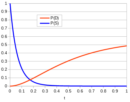
Making a plot of the two parts of the equation we can see that the probability that two sites are the same goes down as the time of divergence increases and the probability that they are different increases.
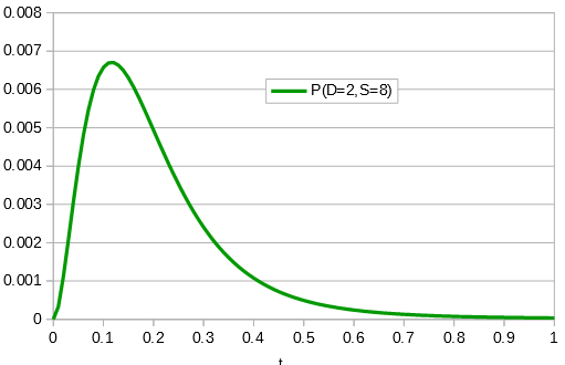
Importantly, there is a middle ground that can best accommodate both signals from the data, the differences and the similarities, near but lower than the crossover point. Combining these together we get the curve of probability of all the data with a peak just above 0.1.
This can be integrated to find upper and/or lower confidence intervals (which is messy and uses the hypergeometric function); however, it is clear from looking at the curve that a wide range of values are hard to rule out with a data set this small.
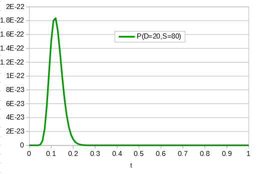
If the data set were larger we can narrow down the confidence interval.
So, how does this compare to the point estimate we get from the traditional Jukes-Cantor distance? A difference of 0.2 (two sites out of 10) can be plugged in for  ,
,
 ,
,
and gives  .
.
When we take the derivative of

set it equal to zero and solve for  we get
 .*
.*
Plugging in  and
and  gives
gives  , exactly the same as with the other method. The original Jukes-Cantor method is a maximum likelihood point estimate (the parameter value of the model that maximizes the likelihood of the data). You can also see it is equivalent in other ways. The
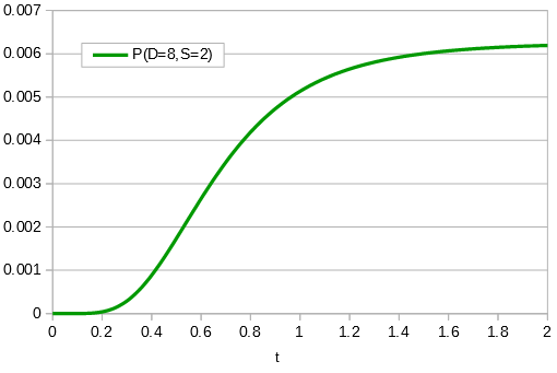
  in the denominator makes the log evaluate a negative number if the fraction of sites that vary are greater than 3/4 of the total, which is undefined. (Thinking about this intuitively it is most consistent with positive infinity; however, I suspect the curve gets infinitely flat and almost any large number is essentially just as likely.) However, we can still work with the probabilities which allows us to rule out small values of
  as in the example below where the sites that differ are 80% of the total.
* This is only true for real solutions. The more general solution is
 ,
,
where  is an element of the integers. This is fun because it combines a base
  log with
  and
and  , but this isn't really relevant to the discussion (time of divergence doesn't rotate into a second dimension).
