In the last mutation model posts I talked about irreversible and reversible mutations between two states or alleles.  However, there are four nucleotides, A, C, G, and T.  How can we model mutations among these four states at a single nucleotide site?  It turns out that this is important to consider for things like making gene trees to represent species relationships.  If we just use the raw number of differences between two species' DNA sequences we can get misleading results.  It is actually better to estimate and correct for the total number of changes that have occurred, some fraction of which may not be visible to us.  The simplest way to do this is the Jukes-Cantor (1969) model.

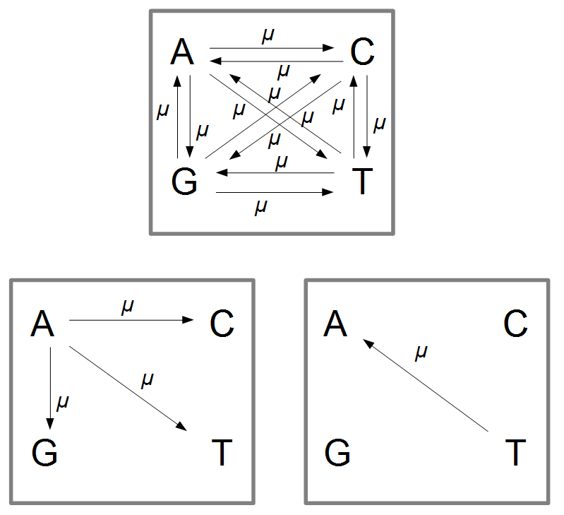
Imagine a nucleotide can mutate with the same probability to any other nucleotide, so that the mutation rates in all directions are equal and symbolized by μ.

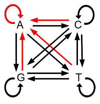
So from the point of view of the "A" state you can mutate away with a probability of 3μ (lower left above).  However, another state will only mutate to an "A" with a probability of μ (lower right above); the "T" could have just as easily mutated to a "G" or "C" instead of an "A".

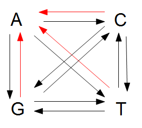
When we talked about the reversible mutations one result was that the equilibrium frequency of a state was the rate of mutation to that state divided by the total rates of all mutations.  We can see above that there is one μ moving toward "A" from a specific state and 3μ moving away.  This gives 1μ/(3μ+1μ) or 1/4 as the predicted frequency of "A" in a DNA sequence at equilibrium, which makes sense, if mutations occur in all directions at equal frequencies then we expect 25% of the nucleotides to consist of "A's".  This is also true if we look at all the possible mutations simultaneously.

There are three paths to "A" and nine other paths for a total of 12.  3/12=1/4.

Now it's time to talk about the Poisson distribution.  This is a convenient distribution to use in many cases where the probability of an individual event is rare, events occur independently, and we are thinking about intervals of continuous time (or space).  Classic examples are the number of people in a line at the bank per hour, or the number of letters received in the mail per day, or the number of Prussian soldiers killed each year by horse kicks, or less classic, for example, the number of meteors larger than 10 meters in diameter that impact Earth's atmosphere each decade (this happens to be slightly less than one on average).

The probability of each number, , of events can be calculated given the average expected number, , according to:

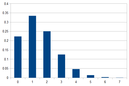
So, if on average we expect events, the probability of zero, one, two, etc. events looks like this:

In words, the probability of no events is 22.3%, one event is 33.5%, two events is 25.1%, three events (twice the average) is 12.6%, ... seven events is less than 0.1% and the probability of eight or more events, given the average is 1.5, is practically zero.

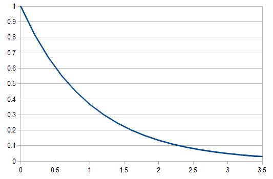
Of special interest is the probability of no events, .  Then the equation simplifies to:

So, as the mean increases (x-axis below) the probability of zero events (y-axis) drops according to an exponential distribution.

By definition, the total probability of all possible outcomes must sum to one, "something has to happen, even if it is nothing."  So the probability of one or more events (at least one event) is one minus the probability that it did not mutate, which is the probability complement of , which can be written as (the probability that there are not zero events given the expected number of events):

To bring this back to mutations, we expect some number of mutations to occur over an interval of time.  So we multiply the mutation rate, , by time, , to get an expectation. Starting at one site, there are three possible paths moving away, so there are three opportunities for mutation, so it seems that each time step the mutation rate is .

However, for mathematical convenience we are going to add a strange possibility.  It is easier to work backwards and say if the site did mutate at least once, the probability it mutated to a "G," for example, in the last step is 1/4, no matter how many total mutation steps occurred.  But this is not true under the model we drew above if the site was a "G" before mutating.  The same state can not mutate to the same state, or it wouldn't be a mutation as we understand it.  Anyway, let's allow for the time being the possibility that a site can "mutate" back to itself, also at rate μ.  So we get a visual model like this:

Now the potential for mutation each time step is .

This is the mean of the Poisson, .

Actually there is a 2X correction.  The DNA sequence is inherited from a common ancestor along each lineage to each modern species that we are comparing.  So the actual distance in twice the time to the common ancestor.  .

So, the probability of a DNA site not mutating between two species is

The probability of at least one mutation is:

Now, in our modified model, if there has been at least one mutation, the probability you end up at a specific state like a "T" is 1/4.  Combining these we get (say we started with an "A"):

In fact, ending back at an "A" is also:

The probability that the same site is different in the two different species is:

Because, with one species at one state at a site there are three possibles ways to be different in the other species, and to do this at least one mutation had to occur between them.

We can see the equilibrium distance from the equation.  raised to a large negative value approaches zero.  and this one is multiplied by .  So at equilibrium the distance between two sequences, that began as identical, is 75%.  In other words, just by chance 1/4 of the sites will happen to match because there are four nucleotides to choose from.

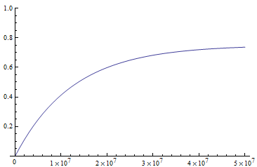
If we plug in realistic mutation rates, like we get this kind of curve.

The x-axis major units are 10 million generations (or time units).  The trajectory is near equilibrium at 50 million generations.  Also, the per nucleotide mutation rate is much smaller than the per gene mutation rate where there are many more nucleotide sites that can disrupt the gene.

Ok, so our expected distance (), the fraction of nucleotides that are different, is

What we really want in species comparisons is a measure that is linear with time.  Let's set , which is time linear, substitute it in and solve.

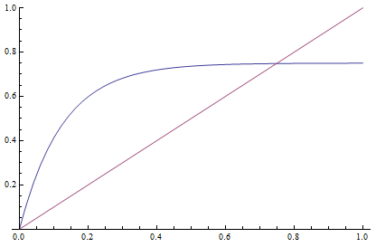
This takes the raw distance (blue curve below) and converts it (assuming the mutation model is a reasonable approximation) into a time linear distance between species (red line below).

If you look up the Jukes-Cantor distance correction in other places you may see different numbers.  This is because there are different ways to scale mutation when you write down the model.

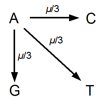
One approach is to divide all the mutation rates by three (μ/3), so that the total rate of mutation away from a state is μ.  This seems reasonable and gives

Another common variation is to ignore the X2 correction for two lineages from a common ancestor and just think of it as a single lineage from a common ancestor, which gives:

This last "3/4,4/3" version above is the most common way of writing the Jukes-Cantor model correction in the literature.  Of course 1/4 of the estimated total number of mutations are not really mutations as we normally think of them because they result in the same nucleotide state. If I were pressed I guess I would say the "best" estimate, in terms of intuitive definitions of mutations, of the actual number of mutation events that have occurred based on the difference of two sequences is 3/4 of the μ/3 rates with the X2 time correction:

.

This is an estimate of events over time, based on our model, that we would actually call mutations--I think. However, in the end it doesn't really matter how mutation and time are scaled as long as it is consistently applied between comparisons.  What we really want is a distance measure, from the fraction of differences out of the total, that is proportional to () the mutation rate and time (the slope doesn't matter so long as it is linear) rather than to try to directly estimate the actual number of mutations that have occurred over the time period:

If we also assume mutation rates are constant, this is simply time linear:

OK, that's enough for now.  Later I want to talk about how this connects back to the discrete time model for reversible mutations and look at an example of using this.