We've taken another big step forward recently.  We are now microinjecting Culex mosquito embryos with genetically modified transposable elements that can potentially integrate into their genome.  We are starting with a test system to save time.  I cloned, grew, and isolated two plasmids (kind of like small artificial chromosomes) in E. coli bacteria that have a piggyBac transposable element system (originally from a species of moth, Trichoplusia ni).  One plasmid (the "helper" plasmid) is immobilized but produces the transposase enzyme that can integrate DNA into the genome.  The other "donor" plasmid is mobile with flanking piggyBac sequences but does not produce its own transposase (Wimmer 2003).  Instead it contains GFP (green fluorescent protein, originally from Aequorea victoria jellyfish) under an artificial 3xP3 "eyeless" promoter that should express in the eyes (which may be occluded by pigments) and larval optic nerve (Sheng et al. 1997; Berghammer et al. 1999).  Here is an image of the two isolated plasmids run on a gel.

The first two lanes to the left show the plasmids and the third lane is a "ladder" to measure sizes.  The lowest band is a supercoiled plasmid.  The higher bands are plasmids that have single strand or double strand breaks in the DNA sequence (and so are less compacted and run slower through the gel).

We loaded the plasmids in the microinjection needle and injected newly laid eggs.  This was a trial run to get the system worked out (injection pressure, egg age timing, slide set up, etc.).  Some of the mosquitoes survived the procedure and were large enough for us to take a good look at them this week under the microscope.  We don't really expect this first batch to contain any genetically modified individuals, although it is possible.  However, even if some cells contained insertions the individual would be a genetic mosaic and may not be transformed in the germ line.  The next generation offspring are the real test.  At this point we are establishing more of a baseline of what the larvae look like.

First of all, here is a larvae under normal light.

We are interested in the pattern of fluorescence under higher energy / bluer light.  This is what they look like in that case.

You can see some red and green autofluorescence.  Part of this probably results from the food we give the larvae which shows up as flecks of green and red in the water---the reason to establish this kind of baseline.  Here is the type of pattern (from another mosquito species) behind the eyes (green lines) that we would expect with a 3xP3-EGFP transformation:

In the following images I turned up the regular light a bit so that they are under both light sources.

We will let you know how the next generation turns out...

Berghammer, A. J., Klingler, M., & Wimmer, E. A. (1999). Genetic techniques: a universal marker for transgenic insects. Nature, 402(6760), 370-371

Sheng, G., Thouvenot, E., Schmucker, D., Wilson, D. S., & Desplan, C. (1997). Direct regulation of rhodopsin 1 by Pax-6/eyeless in Drosophila: evidence for a conserved function in photoreceptors. Genes & Development, 11(9), 1122-1131.

Wimmer, E. A. (2003). Applications of insect transgenesis. Nature reviews genetics, 4(3), 225-232.

This post is two weeks out of order but Brian Deis had a surprise for us on Halloween.

Brian came as my twin "Loyd Reed" on his name tag.  He had a fake beard, glasses, Hawaiian shirt, shorts, belt and flip-flops ("slippers" here in Hawai'i) to match and even tried to part his hair in a similar way.  He was in one of my classes later in the day so I sat in the audience at first and he was up "on the stage" when people walked in.  He created a lot of smiles around the department.

I have to apologize for stealing the photo from one of Jolene's blog posts:

https://sites.google.com/site/jolenesutton/current-research/Research-Blog/itisntallworkandnoplayinthebiologydepartment

The irony to this is that, unkown to Brian, I am named after my grandfather Floyd that in fact had an identical twin named Lloyd.

Our own Aki Laruson and Caitlyn Genovese from the Moran lab were interviewed yesterday by Jay Fidell in a "Research at UH Manoa" segment on "ThinkTech Hawai'i".  Here is the YouTube link

and the descriptive blurb:

Research at UH Manoa
Understanding Urchins
Research at UH Manoa, with graduate students Aki Laruson and Caitlyn Genovese

Sea urchins, called wana in Hawaiian, are common on the rocks and reefs surrounding our islands. UH Manoa graduate student Aki Laruson is working to identify patterns of genomic divergence in so-called "collector" urchins, Tripneustes sp. These are the urchins that have been put to task to help control invasive seaweed growing in Kaneohe Bay. Caitlyn Genovese is studying growth energetics in marine invertebrate larvae including the local urchin population. Together they are using a variety of techniques ranging from phylogenetics to ecology to population genetics to bring new light to the evolutionary relationships of this pantropical species.
When
Mon Nov 10, 2014 1pm – 2pm Hawaii Time

To be honest, I was troubled by the hosts references to homeless children, "urchins," at the beginning of the interview, but Aki and Caitlyn both did a great job!

Some more info about urchin etymology from Google:

I have been teaching myself R lately and had an idea for a simulation the other night so I've been working on this...

Many of us are familiar with the idea that eventually a room full of monkeys with typewriters will type the complete works of Shakespeare (the so-called infinite monkey theorem).  This has been used as an argument to illustrate ideas of biological evolution.  However, it falls far short.  The infinite monkey theorem works well for the intuition of random mutations, but it does not illustrate the power of selection and recombination to enrich the frequency of closer matches to a given text in a population (for mutation then to act upon).

I wrote a script to try to illustrate this and evolved seven random letters to the word "Brevity."  This used random mutation, assigned relative fitness values to the sequences based on how many letters matched "Brevity," and recombined sequences randomly in the population.  Here is a plot of how the simulation preformed.  The average fitness in the population is shown by the blue line, the maximum fitness over all sequences is the upper line in the plot and the minimum fitness is the lower line.  Examples of the maximally and minimally fit sequences are given above and below the plot every ten generations.

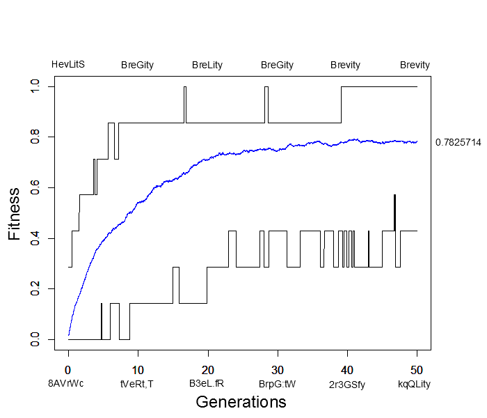
This simulation was based on 500 sequences (or the equivalent of 250 diploid individuals) with a per generation, per character mutation rate of 2% and a per generation, per sequence recombination rate of 50%.  In less than 40 generations the population contained perfectly matching individuals spelling out "Brevity" from a starting best match of "HevLitS" in the first generation.  However, the population appears to have reached an apparent fitness equilibrium of close to 80% and poorly matching (40% fitness) sequences such as "kqQLity" remain at generation 50.  This is much sorter than the complete works of Shakespeare; however, it is also clear that the target "Brevity" was arrived at much faster with selection in a population than by just random mutation.

In fact, the target sequence was arrived at a couple of times, even briefly before 20 generations, but then disappeared again before the longer term arrival at 40 generations.  This illustrates one result of population genetics, that even though a new mutation may be more fit than any other versions (alleles) in the population, it is actually more likely to be lost by genetic drift (evolutionary sampling error) in the following generations than to increase dramatically in frequency.

What would happen if the simulation were allowed to run for much longer, say 500, 5,000 or even five million generations?  Would the average fitness eventually reach 100% with the entire population made up of the target "Brevity" (with the occasional rare mutation of course)?  An easier way to answer this than running the simulation for a very long time is to start the population with all perfect matches and see how closely it remains at this peak starting point.  Here is the result (under the same parameter values as the simulation result above):

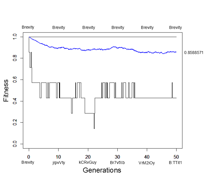
Immediately the average fitness drops dramatically with sequences like "jrpvVty" appearing by generation 10.  At generation 50 the population arrives at a fitness near 85% of the maximum possible with lower bound fitnesses of 40%.  This is not far away from the near 80% arrived at before (also with a lower bound of 40%).  This illustrates the concept of "mutational load" in a population---that the average fitness will be quite a bit less than the theoretical maximum at mutation-selection equilibrium.  It takes time for deleterious mutations to be purged by selection and the net effect is a sizable reduction in fitness, in the case an average reduction of 15% to 20% from the maximum possible.

I am planning to continue discussing this in a few more posts.  This simulation might be a good way to illuminate the effects of population size,  mutation rates, recombination rates, and genome size on the evolutionary trajectory of a population.

While making this post I also inadvertently learned about a similar simulation called the "weasel program" by Richard Dawkins.  However, there are some important differences in the algorithm.  I also plan on discussing some ways the process of selection can be simulated---I came across some alternatives to the way natural evolution is typically modeled that dramatically change the trajectory of average population fitness, including the framework used by Dawkins.

Here is the R source code if you want to play around with it yourself:

# output the results to a text file if printout set to 1, 0 otherwise
# you should change the path to match your directory structure
# (it runs faster without the text output)
printout=1
if(printout){
  sink("C:\\Users\\Floyd\\Desktop\\backup\\work\\typewriter\\monkey_type_7_out.txt", 
    append=TRUE, split=TRUE)
}

length=7 # sequence length
n=500 # number of seequences
mut=50 # inverse mutation rate, one out of #
rec=2 # inverse recombination rate, one out of #
step=n*50 # "generations" in a Moran model

# store the population of sequences
pop=matrix(0,nrow=n,ncol=length)
# a vector of sequences
fit=matrix(0,nrow=n,ncol=1)

# set initial random sequences
for(i in 1:n){
  x<- sample(c(0:9, letters, LETTERS," ",".",",",":"),
             length, replace=TRUE)
  pop[i, ]=x
}

# keep track of fitnesses and generations during the run
runbestfit<-numeric() # best fitness
runavefit<-numeric() # average fitness
runleastfit<-numeric() # least fit
rungen<-numeric() # generations

target<-"Brevity" # target sequence

# divide into characters in a matrix for testing
targ<-strsplit(target, "")
t<-matrix(unlist(targ))

# if(1) sets population to all match target for testing
# if(0) turns this off
if(0){
  for(j in 1:n){
    for(i in 1:length){
      pop[j,i]=t[i]
    }
  }
}

# loop through time steps
for(s in 1:step){

  rungen[s]=s/n # generations defined as n time steps

  badfit=length
  badfitind=1
  maxfit=0
  maxfitind=1
  matchsum=0
  # loop through each position and add up if a match exists
  for(j in 1:n){
    match=0
    for(i in 1:length){
      if(t[i]==pop[j,i]){match=match+1}
    }
    matchsum=matchsum+match
    if(match>maxfit){
      maxfit=match
      maxfitind=j
    }
    if(match<badfit){
      badfit=match
      badfitind=j
    }
  }
  bestexample<-paste(pop[maxfitind,], collapse="")
  worstexample<-paste(pop[badfitind,], collapse="")
  runavefit[s]=matchsum/(n*length)

  # report current status
  if(printout){
    print(paste(s/n, "best ", bestexample))
    print(paste(s/n, "worst", worstexample))
  }

  #pick random individual to copy from weighted by relative fitness
  randfitpoint=sample(matchsum,1)
  repind=1
  matchsum=0
  for(j in 1:n){
    match=0
    for(i in 1:length){
      if(t[i]==pop[j,i]){match=match+1}
    }
    matchsum=matchsum+match
    if(matchsum>=randfitpoint){
      repind=j
      break
    }
  }

  # pick random individual to be replaced
  pick=sample(n,1)
  for(i in 1:length){
    pop[pick,i]=pop[repind,i] # best way to represent natural population (?)
  }

  # add mutations to the replicating sequence
  for(i in 1:length){
    m=sample(mut,1)
    if(m==1){
      x<- sample(c(0:9, letters, LETTERS," ",".",",",":"),
                   1, replace=TRUE)
      pop[pick,i]=x
    }
  }

  # add recombination with another sequence to the replicating sequence
    r=sample(rec,1)
    if(r==1){
      another=sample(n,1)
      location=sample(length,1)
      for(i in location:length){
        temp=pop[pick,i]
        pop[pick,i]=pop[another,i]
        pop[another,i]=temp
      }
    }

  # update best and least fit
  runbestfit[s]=maxfit/length
  runleastfit[s]=badfit/length

  # update plot of results
  # only every 50 time steps so it doesn't run too slowly
  if(s%%50==0){
    plot(rungen,runbestfit,type="l",xlab="generation",ylab="fitness",ylim=c(0,1))
    par(new=T)
    plot(rungen,runavefit,type="l",col='blue',xlab=" ",ylab=" ",ylim=c(0,1))
    par(new=T)
    plot(rungen,runleastfit,type="l",lwd=0.1,xlab=" ",ylab=" ",ylim=c(0,1))
  }

  # report current average fitness
  if(printout){print(runavefit[s])}
}