The binomial distribution that many of us are more familiar with is a special case of the multinomial distribution, which can have more than two outcomes to a "test". is a common summary of how similar populations are on a genetic level and it is based on the concept of "missing heterozygosity". I was thinking of a way to illustrate the multinomial with the probabilities of genotypes under Hardy-Weinberg assumptions, an allele frequency, , and the degree of missing heterozygosity, .

Here is a small dataset to work with, counts of three genotypes of a SNP with two allelic states in a sample of 30 individuals.

• AA  4
• AT  10
• TT  16

We can go back to the binomial for a moment and estimate the allele frequency. If we ignore genotype (the association between alleles), there are 18 A's and 42 T's.

• A  18
• T  42

So 30% of the alleles are A alleles. With the binomial, the probability of the data given an allele frequency is

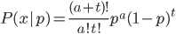
where is the number of A alleles and is the number of T alleles.

Plot this in R to visualize the probability of the data given the range of possible allele frequencies.

a=18
t=42
n=a+t
p <- seq(0,1,length=1000)
probx <- dbinom(a,n,p)
plot(p, probx, type='l',xlab="allele frequency", ylab="probability",
     main="Binomial Probability")

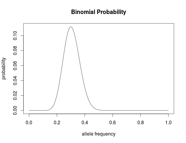
We can find the maximum likelihood point by finding the partial derivative (slope) with respect to , setting it equal to zero, and solving for . First of all the binomial coefficient in the front is a constant so we can remove that for simplicity.

Let's define as the sum of and .

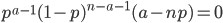
This makes intuitive sense. The best guess for the allele frequency is the number of times it is observed out of the total.

We can also integrate to get the area under the curve. The indefinite integral is

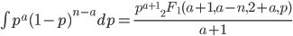
is the ordinary hypergeometric function. First this has to be evaluated at to put it on a scale where the area under the curve sums to one. For and this comes out to .

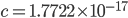Evaluating

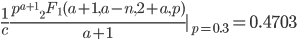
at the maximum likelihood point, , gives a cumulative probability of 0.4703, which is not far from 0.5, the median of the distribution. You can evaluate it online with this link to Wolfram Alpha:

https://www.wolframalpha.com/input/?i=(0.3%5E19*hypergeometric2f1(19,-42,20,0.3))%2F(19*1.7722*10%5E(-17))

Evaluating

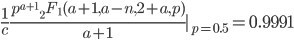
at for example gives a cumulative probability of 0.9991; so, more than 99% of the curve is below this point and we can say that is significantly less than given the data.

Okay, that was a warm up; now let's do this with the genotypes before adding in .

Going back to the original genotype dataset of 30 individuals.

• AA  4
• AT  10
• TT  16

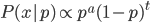
The multinomial probability is

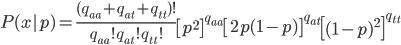
where are the counts of each genotype in the sample and is still the frequency of allele "A."

We can plot this along with the binomial curve for comparison with the following Mathematica code.

aa = 4;
at = 10;
tt = 16;
a = 2*aa + at;
t = 2*tt + at;
Plot[{Multinomial[aa, at, tt] (p^2)^aa (2 p (1 - p))^at ((1 - p)^2)^
    tt, Binomial[(a + t), a] p^a (1 - p)^t}, {p, 0, 1} , 
 PlotRange -> Full, PlotLegends -> {"Multinomial", "Binomial"}, 
 AxesLabel -> {"p", "P(x)"}]

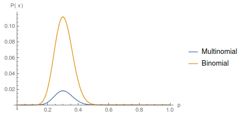
The curves are similar, they peak in the same place, but overall the multinomial curve has a lower probability than the binomial. This is because there is more information in the multinomial. Each set of the data for the binomial (allele counts) can correspond to a range of ways to divide the data into genotype counts. We can always reduce genotypes to number of alleles but we cannot do the reverse. So, a particular genotype outcome is less likely (a smaller part of all possible outcomes) than the corresponding allele count outcome.

Okay, now it gets a little more fun. We have a probability over a dimension of allele frequency of from zero to one. Let's add another dimension of but first let's think about what means. is the proportion of expected (according to Hardy-Weinberg) heterozygosity that is missing. The heterozygous genotypes don't just disappear. The alleles get reorganized into homozygous genotypes. The frequency of each allele in the heterozygotes is 1/2; so, each homozygous genotype is increased by an equal proportion, which is half of the heterozygotes that are missing. Thus, the frequency of each genotype expected given and is

This can be incorporated into the individual genotype probability components of the multinomial.

We can simply the frequency of each genotype terms by symbolizing then with corresponding terms.

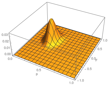
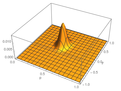
This is what the likelihood surface looks like over the range of from zero to one and from zero to one.

Here is the mathematica code used to make the plot.

a = 4;
h = 10;
t = 16;
Plot3D[Multinomial[a, h, t] (p^2 + f p (1 - p))^
   a ((1 - f) 2 p (1 - p))^h ((1 - p)^2 + f p (1 - p))^t, {p, 0, 
  1}, {f, 0, 1}, PlotRange -> Full, AxesLabel -> {"p", "F", ""}, 
 PlotPoints -> 100]

The curve at corresponds to the multinomial curve above (in the plot comparing it to the binomial). We can also see that allowing positive values for can result in higher likelihoods of the data. What do we actually expect to be? The number of heterozygotes are 10 out of a sample of 30 genotypes, so the fraction of heterozygous genotypes is 0.333. The allele frequency is 0.3, so we expect of the sample to be heterozygous. There is a 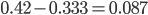proportion of heterozygotes that are missing. This is 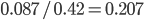of the heterozygosity expected. So our point estimate of is 0.207, or about 21% of the heterozygosity is missing. This appears to correspond to the top of the likelihood peak. Finally, notice that the peak is narrower in the dimension than in the dimension. There is more information in the dataset about the allele frequency than there is about the genotype frequencies. There is a larger sample, 60, of alleles than there are of genotypes, 30. So, the estimate of is more refined than the estimate of .

The range of zero to one makes sense for . An allele frequency cannot be less than zero or greater than 1. Also, cannot be more than one (all of the expected heterozygosity is missing), but it can be less than zero (negative means there is an excess of heterozygosity). It looks like a large volume of the likely values of and given the data correspond to a negative . So, is not significantly greater than zero (Hardy-Weinberg expectations) for this dataset. Let's extend the plot to encompass a range of negative values for .

...and something weird happened. There is a second likelihood peak with different values of and that actually has an even higher likelihood at its peak, but the parameter values are unreasonable (given what we can see in the dataset about the allele frequency and level of heterozygosity). The minimum possible is negative one. If the entire sample were made up of heterozygotes then the allele frequency is one half, the proportion of heterozygotes expected would also be one half. This leads to a negative one half divided by one half or negative one. Extending the plot out to the full range looks even more pathological (I limited the scale and truncated the peak because it was so large).

Long story short it turns out that this is an artifact... If you closely inspect what is going on by spot checking a few points in the second peak you find that the expected number of the rarer homozygote is negative, which is impossible, and in the likelihood calculation this is raised to the fourth power, which makes it positive, etc. This is a good example of how unanticipated, and initially cryptic, errors can creep into a computational script. This is fixed by setting up an if statement to only evaluate the likelihood if the expected number of homozygotes are positive; otherwise the likelihood is zero, which is true. Here is the updated script and a plot.

a = 4;
h = 10;
t = 16;
Plot3D[Multinomial[a, h, t] If[
   p^2 + f p (1 - p) > 
    0, (p^2 + f p (1 - p))^a ((1 - f) 2 p (1 - p))^
     h ((1 - p)^2 + f p (1 - p))^t, 0], {p, 0, 1}, {f, -1, 1}, 
 PlotRange -> Full, AxesLabel -> {"p", "F", ""}, PlotPoints -> 100]

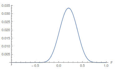
Because and appear uncorrelated we can feel good about taking a slice of the likelihood surface through the maximum-likelihood value of as a reasonable approximation of the (contour) likelihood surface of in order to evaluate the range of possible parameter values.

This is not yet . We have been evaluating the missing heterozygosity of a single population sample. Heterozygosity can be reduced within a population by inbreeding effects where individuals do not mate randomly but tend to mate more often with closer relatives (selfing in plants is an extreme example). What was calculated above is .

Let's say we had another sample from a different population. So now we have our original population one

• AA 4
• AT 10
• TT 16

and population two.

• AA 10
• AT 14
• TT 6

Plotting the likelihood surfaces together.

a1 = 4;
h1 = 10;
t1 = 16;
a2 = 10;
h2 = 14;
t2 = 6;
Plot3D[{If[p^2 + f p (1 - p) > 0 && (1 - p)^2 + f p (1 - p) > 0, 
   Multinomial[a1, h1, t1] (p^2 + f p (1 - p))^
     a1 ((1 - f) 2 p (1 - p))^h1 ((1 - p)^2 + f p (1 - p))^t1, 0], 
  If[p^2 + f p (1 - p) > 0 && (1 - p)^2 + f p (1 - p) > 0, 
   Multinomial[a2, h2, t2] (p^2 + f p (1 - p))^
     a2 ((1 - f) 2 p (1 - p))^h2 ((1 - p)^2 + f p (1 - p))^t2, 0], 
  0.0005}, {p, 0, 1}, {f, -1, 1}, PlotRange -> Full, 
 AxesLabel -> {"p", "F", ""}, PlotPoints -> 100]

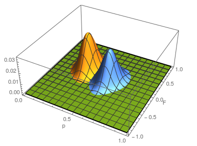
The second sample has a higher allele frequency and a value of closer to zero (however, the two ranges of likely values overlap and might not be considered significantly different). The second allele frequency is . With the two allele frequencies we can now calculate a point estimate of between the population samples. The expected heterozygosity in sample 2 is . We already showed above that and . The average allele frequency over both populations is and the average subpopulation expected heterozygosity is . In a combined total sample, if there were population structure, the expected heterozygosity is 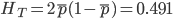. Therefore,

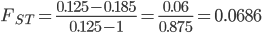
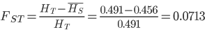
or about 7% of the expected heterozygosity is missing because of differences in allele frequencies between the populations. Why does this work? Any time there is a difference in allele frequency the average subpopulation expected heterozygosity will be lower than the combined expected heterozygosity. Why? Because the curve of heterozygosity over allele frequency space is a concave function; the average of two points will always be lower than the value of the function evaluated at that point.

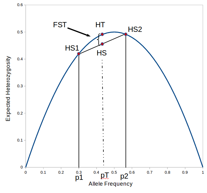
is the gap between and , which is 7% of .

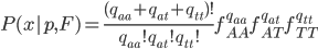
Before bringing this back together I need to introduce one more -statistic. This one is . It is the total missing heterozygosity due to both population structure and inbreeding effects. If we combine the two samples we get

• AA 14
• AT 24
• TT 22

The allele frequency (the same as the average between the two samples) and the fraction of heterozygotes in the combined sample is 40%. We expect a heterozygosity of 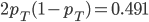. So, .

between populations is related to and . If we know the latter two we can estimate the former.

Using an and let's say an we get

.

We can estimate and using the multinomial, which means we can also estimate . This is starting to get more complicated with lots of parameters to estimate from the data, two allele frequencies and two statistics (if we have a single over both populations, which seems biologically reasonable) or four parameters in total. A good way to explore higher dimensional parameter space is to use a Markov Chain in a Monte Carlo fashion (MCMC) with Metropolis-Hastings algorithm. I save the details of this method for a later post. For now let's write a "hill climbing" Monte Carlo script (Monte Carlo refers to guessing parameter values and hill climbing means that it moves to values that produce higher probabilities of the data). Here it is in R.

# data
pop1=c(4,10,16)
pop2=c(10,14,6)
popt = pop1 + pop2

# intialize variables
probbest = 0
p1best=0.5
p2best=0.5
fisbest=0
fitbest=0

# loop through some steps
for (i in 1:100000) {

  tune = 1/i # narrows in as the run goes
  
  # pick new parameter values and check to make 
  # sure they are not out of bounds
  p1 = p1best + runif(1, min = -tune, max = tune)
  if (p1<0) {p1=0} else if (p1>1) {p1=1}
  p2 = p2best + runif(1, min = -tune, max = tune)
  if (p2<0) {p2=0} else if (p2>1) {p2=1}
  fis = fisbest + runif(1, min = -tune, max = tune)
  if (fis< -1) {fis= -1} else if (fis>1) {fis=1}
  fit = fitbest + runif(1, min = -tune, max = tune)
  if (fit< -1) {fit= -1} else if (fit>1) {fit=1}
  pt = (p1+p2)/2

  # genotype probabilities
  gp1=c(p1^2+fis*p1*(1-p1),2*p1*(1-p1)*(1-fis),(1-p1)^2+fis*p1*(1-p1))
  gp2=c(p2^2+fis*p2*(1-p2),2*p2*(1-p2)*(1-fis),(1-p2)^2+fis*p2*(1-p2))
  gpt=c(pt^2+fit*pt*(1-pt),2*pt*(1-pt)*(1-fit),(1-pt)^2+fit*pt*(1-pt))

  # sample probabilities
  if(p1^2+fis*p1*(1-p1)>0 & (1-p1)^2+fis*p1*(1-p1)>0) {
    prob1<-dmultinom(pop1, , gp1)
  } else {
    prob1 = 0
  }
  if(p2^2+fis*p2*(1-p2)>0 & (1-p2)^2+fis*p2*(1-p2)>0) {
    prob2<-dmultinom(pop2, , gp2)
  } else {
    prob2 = 0
  }
  if(pt^2+fit*pt*(1-pt)>0 & (1-pt)^2+fit*pt*(1-pt)>0) {
    probt<-dmultinom(popt, , gpt)
  } else {
    probt = 0
  }
  # combined probabilities
  prod = prob1 * prob2 * probt

  # keep the best ones
  if(prod>probbest){
    p1best=p1
    p2best=p2
    fisbest=fis
    fitbest=fit
    probbest=prod
  } else {
    p1 = p1best
    p2=p2best
    fis = fisbest
    fit = fitbest
  }
  pt = (p1+p2)/2

  # calculate fst
  fst = (fis-fit)/(fis-1)

  # report results
  print(c(p1,p2,fis,fit,fst))
}

Running this for 100,000 steps I got estimates of , , , , and ; not bad.

Okay, that's going to have to be it for this post. This could be extended to cases where the sample sizes are unequal, multiple loci ( is shared across loci but is not), more than two alleles, more than two populations and hierarchical population groupings, and an MCMC script to estimate the probability distribution of , but I'll have to save that for later.