There are several ways to model or simulate genetic drift (random changes in allele frequencies) in a population over time.  Some of the simplest and most direct are 1) binomial sampling and 2) forward simulations, where every allele copy is kept track of in every generation.  However, these more complete approaches can be very slow (computationally intensive) with large populations over many generations.  Another approach is a 3) diffusion approximation that generates a probability distribution of allele frequencies at a given time point.  Yet another widely used approach is the 4) coalescent.  Coalescent simulations are very efficient because they only track the ancestral lineages of a sample of allele from the population (most allele transmission events can be ignored because they do not contribute to the last generation).

I have worked with all of these approaches in one form or another and they all have pluses and minuses that depend on the question being asked.  The diffusion approximation has generated many insights into population genetics; however, in generating outcomes (say for simulation) it can be inefficient.  The probability distribution is generated by a sum of a series of Gegenbauer polynomials, and these are slow to converge.  I was thinking about this recently and wondered if the diffusion approximation could itself be approximated by a beta distribution.  This might be more computationally efficient.

Beta distributions have two parameters, and .  The mean (expectation) of a beta distribution is .  In genetic drift, if we imagine a large number of populations drifting away from the same starting allele frequency, the average allele frequency across all of these populations is not expected to change.  Genetic drift does not push allele frequency change in a direction.  Alleles are just as likely to increase or decrease in frequency.  So, if we have as the initial allele frequency then we expect 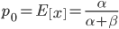and that this remains constant over time.  Incidentally, you might also see that 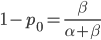because these are both fractions out of the total.

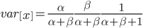
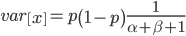
On the other hand, the variance in allele frequencies between replicate populations is expected to increase over time as the populations diverge due to genetic drift.  The variance of a beta distribution is 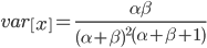.  Right away we can rewrite this as

Under the diffusion approximation the variance in allele frequencies after generations in a population of size diploid individuals is

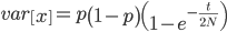
We want to match the variance of a beta distribution to the variance of the diffusion approximation so we can generate beta distributions in terms of the spread of allele frequencies after generations have passed.

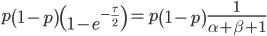
We can cancel out to get

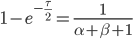
Then rearrange

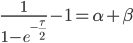
Realizing again that and are fractions out of a total we can define them as

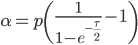
And now we have a beta distribution that is defined in population genetic terms as an approximation to a diffusion approximation.  As a side note, sometimes very "bad" distributions can be used as approximations in population genetics and be surprisingly reasonable.  For example, Kimura used a uniform distribution to model binomial changes in allele frequencies between populations and it works well.  Sometimes a process can be relatively insensitive to underlying distributions.  In another example, Crow worked on a problem of truncating selection and the shape of the area (of the state space) exposed to selection had little effect. (I'll add in some references here later.)

Does this beta approximation work?

Here is a classical result plotted by Kimura (1955, PNAS 41, 144).  It shows the distribution of allele frequencies at a range of generations after starting from .

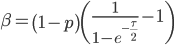
And here is the corresponding beta approximation.

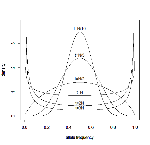
Right away you can see that is is a very good match, especially for short times and intermediate allele frequencies.  The big difference is at the edges.  The diffusion approximation allows for complete loss or fixation of an allele in a finite population.  The beta approximation does not.  An allele frequency can get arbitrarily close to zero or one but variation is never completely lost.  This is why the distribution "stacks up" near the edges.

By the way, I am still working on learning R and used an R script to generate these plots.  Here is the code if you are interested.

driftcoefficient<-function(tau){
  z<-1/(1-exp(-tau/2))-1
  return(z)
}

p<-1/2 # allele frequency
h<-3.8 # upper plot limit

x <- seq(0, 1, length = 1001)

tau<-0.1 # t/N generations
y<-dbeta(x, p*driftcoefficient(tau), (1-p)*driftcoefficient(tau))
plot(x,y,type='l', ylim=c(0,h),xlab='allele frequency',ylab='density')
text(0.5,3.62,'t=N/10')
par(new=TRUE)
tau<-0.2 # t/N generations
y<-dbeta(x, p*driftcoefficient(tau), (1-p)*driftcoefficient(tau))
plot(x,y,type='l', ylim=c(0,h),xlab='allele frequency',ylab='density')
text(0.5,2.53,'t=N/5')
par(new=TRUE)
tau<-0.5 # t/N generations
y<-dbeta(x, p*driftcoefficient(tau), (1-p)*driftcoefficient(tau))
plot(x,y,type='l', ylim=c(0,h),xlab='allele frequency',ylab='density')
text(0.5,1.55,'t=N/2')
par(new=TRUE)
tau<-1 # t/N generations
y<-dbeta(x, p*driftcoefficient(tau), (1-p)*driftcoefficient(tau))
plot(x,y,type='l', ylim=c(0,h),xlab='allele frequency',ylab='density')
text(0.5,1,'t=N')
par(new=TRUE)
tau<-2 # t/N generations
y<-dbeta(x, p*driftcoefficient(tau), (1-p)*driftcoefficient(tau))
plot(x,y,type='l', ylim=c(0,h),xlab='allele frequency',ylab='density')
text(0.5,0.55,'t=2N')
par(new=TRUE)
tau<-3 # t/N generations
y<-dbeta(x, p*driftcoefficient(tau), (1-p)*driftcoefficient(tau))
plot(x,y,type='l', ylim=c(0,h),xlab='allele frequency',ylab='density')
text(0.5,0.35,'t=3N')

Here is another example starting from an initial allele frequency of .

And the beta approximation.

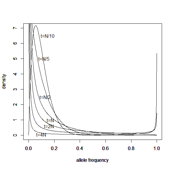
Again, you can see that it does well in the intermediate frequencies and diverges near the boundaries of the distribution.

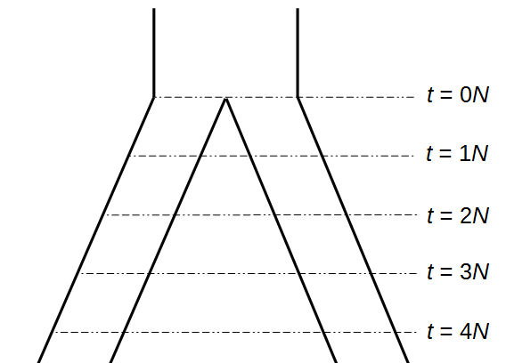
Okay, lets use this beta approximation to play with a model of two populations splitting and evolving over time.  Time is measured in terms of generations after the splitting event.

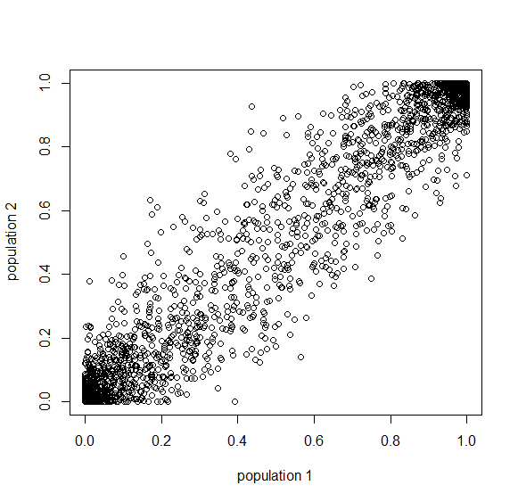
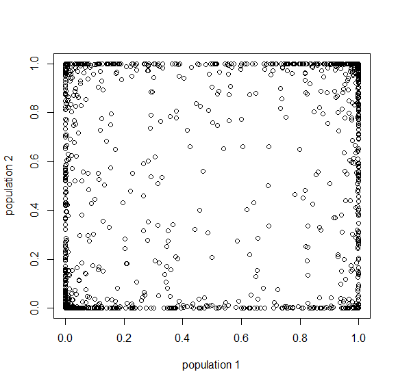
Here is an example of what we might expect to see over time.  The plot below is just generations after the splitting event.  (In human terms we have an effective population size of 10,000 and a generation time of 30 years, so this is about 3,000 years.)

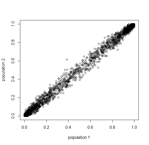
This is from 10,000 randomly generated SNPs (assuming beta-distributed standing variation in the original population).  Most SNPs are near a frequency of zero or one, which is what is typically seen in natural populations.  However, some are at intermediate frequencies.  The SNPs are highly correlated in frequency between the two populations but have begun to diverge.

Here is a plot at generations (30,000 years on a human timescale).

Then generations.

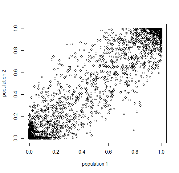
Then generations.

And generations after the division.

A common theme in population genetics is that after generations of genetic drift the initial starting point is essentially lost and an allele that is variable (not fixed or lost) can be at essentially any frequency (a uniform distribution).  You can see this in the distribution plots earlier in this post and can get a feeling for this in the interior of the plot above.

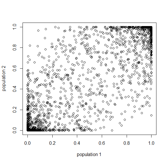
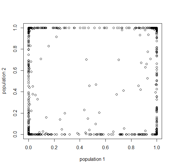
Below is the plot at generations (600,000 years in human time).  Many of the alleles have reached fixation or loss in at least one of the populations.  We are also starting to see alleles that are reciprocally fixed and lost between the two populations (in the upper left and lower right corners).

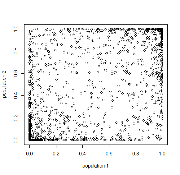
Okay, logically following this we get generations.

Then , where no allele is polymorphic in both populations simultaneously.

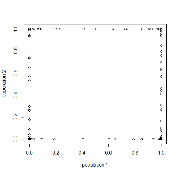
Then , where the starting polymorphism is almost completely lost.

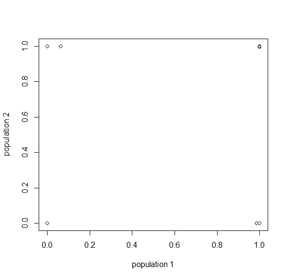
And finally generations results in complete fixation or loss for all 10,000 simulated SNPs.

However, this simulation ignores new mutations that occur over time (which in general will be unique to a population) and gene flow by migration between populations (which will dramatically slow down the divergence between the populations even with small numbers of migrants each generation).  All of these can be added in to elaborate the model.  However, I am pleased that this beta approximation tends to fit general population genetic expectations well.  The problem is with alleles that have almost lost all polymorphism (near the edges of the distribution); however, there is a strong ascertainment bias in population genetic datasets.  For various reasons, we tend to ignore alleles with little variation in favor of alleles that are highly variable across populations, and this is precisely where the beta approximation tends to behave well.  Furthermore, in populations that are connected by gene flow, if an allele is polymorphic in one population it is never really lost (over the long term) in another population.  So perhaps the beta approximation could work well in more realistic scenarios.

Here is the code for the SNP plots in the second half of this post.

driftcoefficient<-function(tau){
  z<-1/(1-exp(-tau/2))-1
  return(z)
}

tau1<-0.01 # t/N generations
tau2<-0.01
snps=10000
thetau=0.05
thetav=0.05
initial<-rbeta(snps, thetau, thetav)
y<-rbeta(snps, initial*driftcoefficient(tau1), (1-initial)*driftcoefficient(tau1))
z<-rbeta(snps, initial*driftcoefficient(tau2), (1-initial)*driftcoefficient(tau2))
plot(y,z,xlab='population 1',ylab='population 2')