Today we did our first trial, preliminary microinjection in the lab!

This is connected to my actual research work and is not just material for the classes I am planning to teach.  We are planning to genetically modify insects by injecting engineered plasmids into multinucleate embryo cells.  I have never done cell microinjections before, and it has a reputation of being quite difficult, so this is one aspect I have been worried about.  However, I have been talking to different people about it, collecting together materials, and we are moving closer step by step.

We now have an inverted microscope set up with a micromanipulator and a "femtotip" glass micropipette needle from eppendorf.  I put some double sided tape (that I picked up at the local Safeway grocery store) on a glass slide and used a paint brush (red sable size one from amazon.com) to place a freshly laid Drosophila egg on the slide (held onto the tape).  Then while looking through the microscope we lined the needle up by moving it through three dimensions by turning different dials on the micromanipulator and poked the tip into the embryo then pulled it back out.  I worked with it a bit then Jolene had a shot at it.

Then I moved a light on the table and the vibrations caused the needle to smash the egg onto the slide...  OK, so it may not seem like much, but I am happy.  There are many more steps to go.  I have two (salvaged) glass needle pullers from making our own needles out of borosilicate capillaries.  However, I ordered commercially made micropipettes for now to keep things simple (but they are expensive).  We also need to set up a positive pressure system to inject the plasmid mixture into the embryos.  This can be done in various ways.  We have an old picospritzer for the line pressure, but when I hook it up to our CO₂ line it vents gas and the pressure gague doesn't budge...?  There may be other alternative however if this doesn't work, for example a DIY picospritzer (link) and Dr. Gert de Couet used to use the faint pressure from turning a thumbscrew in the line to do microinjections.

There is also the preparation of the eggs.  The outer layer needs to be removed (dechrionated with a 1:1 dilution of bleach, that I picked up at the hardware store); they need to be slightly dessicated to absorb the injection without exploding; and, they need to be immersed in oxygen permeable halocarbon oil (I have some halocarbon 700 oil from sigma-aldrich).

Jolene set it up again later on and I got some pictures through the scope (the scope camera doesn't fit into these eyepieces so I just lined up the camera and shot it by hand, sorry about the image quality).

In the image above you can see the glass needle poking into the side of the Drosophila egg.  The needle tip is broken off too large for "real" injections (where we want the embryo to survive) and the embryo is lined up wrong, but this is just a practice run.

We added blue loading dye (used for running loading PCR products to wells in agarose electrophoresis gels) to the needle.  In the image below you can see the dye injected into the center of the egg (faint blue).

In another lab project I am considering for the fall class, I have been experimenting with crossing Sordaria fimicola fungi.  These are molds in the huge phylum of ascomycete fungi that have spores in filaments (asci), which are ordered meiotic products.  So it is an excellent example of meiosis and genetic recombination--if you can get it to work.

In the picture above I have two plates each of wildtype (lower middle and lower right), tan mutants (upper middle and upper right), and gray mutants (upper and lower left) growing from inoculating the center of each plate with some spores.  I had to leave them out on the lab benchtop at room temperature for a few days, so I taped off the area and labeled it in case anyone had any questions about the moldy petri dishes. In the wildtype and tan plates you can see some concentric rings that indicate the temperature fluctuations in the building over the weekend.

In the picture above and below I have set up crossing plates by cutting out cubes of agar containing growing fungi of different types and placing them upside down on the new medium.  You can see the mycelium growing out in a circle from each cube.

Below are older tan and gray mutants that have grown into each other and are crossing.  The darker X at the border looks like wildtype and might possibly be an example of genetic complementation but it is hard to tell if this is not also just denser growth.

And in the plate below is a cross of all three types.  Wildtype in the upper right; tan in the upper left; and gray at the bottom. (Note that the boundaries with wildtype are darker than wildtype alone, which suggests denser growth is at least partially responsible.)

The spores are interesting in this group of fungi because the meiotic products remain oriented relative to each other according to the pattern of chromosome segregation.  The the effects of recombination between the chromosome's centromere and the gene causing the difference in spore color is directly observable.  To illustrate I've diagrammed meiosis in a heterozygote below (these fungi also have a round of cell duplication by mitosis at the end of meiosis resulting in eight spores from each starting diploid cell).

So the reductional division in a heterozygote leads to a 22221111 (or 11112222) pattern of ascospores.  In meiosis I homologous chromosomes segregated (followed by sister chromosome separation in meiosis II) which leads to the four and four ordered pattern.

Below lets look at what happens if there is a recombination event.

Recombination exchanged parts of the homologous chromosomes, so the duplicated alleles were moved to different chromosomes to segregate away from each other.  So in the end the four-and-four pattern is broken up.

In the figure I have shown a 11221122 pattern but this could equivalently have been a 22112211, 22111122, or 11222211 pattern as well as a result of recombination.  The key is that both spore types appear in each half of the asci.  Why does this happen with recombination?  The chromosome segregation (and chromatid separation) are controlled from the centromeres (microfilament fibers attach to the centromeres and they move apart to opposite side of the dividing cell).

In the figures above and below I have indicated condensed duplicated chromosomes joined at the centromere (circle).  The gene's position with the two alleles we can observe is indicated with the line and the alleles with an "A" or "a".  Recombination is indicated by a red arrow.  Distal recombination beyond the gene, away from the centromere, has no effect on what we can observe (above).  However, proximal recombination between the gene and the centromere exchanges the alleles (below).

So as meiosis progresses, the alleles have switched to different (homologous) chromosomes and end up in a different pattern due to recombination.  To try to connect the four different figures above I have drawn it a different way below.

I left out the final duplication of each cell into the eight spores at the end.  (And this is very stylized, cells and chromosomes don't really look anything like this; I'm just trying to get the idea across visually.)

So the frequency of recombinant meiotic products from heterozygotes gives you an idea of how far from the centromere the gene is located on the chromosome.  Normally we count the fraction of recombinants and divide by the total to get the recombinant fraction as a measure of distance.  (This also undergoes a long distance correction for multiple recombination events, but I will talk about that later.)  However, the Sordaria recombinant pattern spores can be a little misleading.  What we are really seeing, usually, is one recombination event out of two possible.  We don't count the non-recombinant spore pattern that is present with the recombinant one in the same asci filament.  So there is a correction-that is easy to forget-where we divide the fraction of recombinant patterned asci by two.

So that is the theory; how about in practice?

The mycelium growing from a spore is composed of masses of thread like hyphae.  These secrete enzymes and absorb nutrients from the environment as they grow.  Essentially the mass, which can sometimes become huge in nature, are all considered a single organism (so when I cut out some agar containing hyphae to set up the cross I essentially cut off pieces of a single fungus to regrow again).  Like mushrooms and many other fungi the mycelium is often hidden in the soil or whatever material the fungus is growing in.  When the hyphae from two different organisms, but within the same species, grow into each other they cross, recombine, and release spores from fruiting bodies like the above ground mushrooms we are familiar with.  In Sordaria the acsi form inside tiny round perithecia (the fruiting bodies) that you smash open with a coverslip in a wet mount on a glass microscope slide.  If you press too hard the asci shear apart; not hard enough and the perithecia are not ruptured.  In addition to this they have to be the right age.  Too young and the perithecia do not rupture easily and the ascospores (spores in the ascus) do not have enough pigment to be able to visualize the genotype.  Too old and the peritheca spontaneously rupture and eject the asci (even before you get to them--this is what they do in nature but in the lab they stick to the inside lid of the petri dish).  When I first tried to look at them they were too young.  Then when I aged them a bit and tried again they were too old and were beginning to coat the lids with spores.  Here are some imperfect pictures from teaching myself how to do this.

Above is a squashed perithicia with a cluster of tan asci beside it.  Below are some darker wildtype spores.

Above you can see both tan mutants and wildtype spore colors, from different perithicia, in the same picture.  Below is a mix of alleles but frustratingly I can't tell how they are ordered or if they are just mixed on the slide.

Below is an example of a bunch of loose spores, which happened all too often.

And finally bingo!

Above is a recombinant meiotic product.  The asci has a 2-2-2-2 pattern of wildtype and gray mutant spore colors.  I've indicated them with arrows below.

The fourth one down appear a bit darker but that is because of overlap with another asci behind it.  I need to keep practicing to get the timing and method down so I can get more useful results with nice flat squashed asci that are not sheared apart.  It was nice to spot a recombinant but I can not yet score enough asci to get data for calculating distance from the centeromere.

In the earlier post about a simple model of reversible mutations I used a discrete time approach.  Events happened in defined time-step generations.  We ended up with something that looked like this to describe the change in frequency over time measured in generations, :

I will leave the details in the earlier post. However, I want to mention that and are mutation rates and I have put a function here to represent the part of the equation that approaches , the equilibrium frequency, as the number of generations, , get large.  Also, we ended up with a difference in allele frequency, when starting at the extremes, and of

My point being that appears a lot.

In the Jukes-Cantor model we used a continuous time approximation to be able to use the Poisson distribution.  So, for example, we had the probability of no mutations occurring along the lineage from an ancestor equal to:

,

where is again the mutation rate per unit time and the total time is .

On the surface these look very different but lets change some things around.

In the Jukes-Cantor model we kept track of four different mutation rates all at a rate of .  In the simple reversible model we kept track of two mutation rates at rates of and .

If we used the form of the reversible model, but used four equal mutation rates, we would have something like:

This is the frequency of the allele that either has not mutated (or has mutated back from another form, which is wrapped up in ).

Let's plot together the probability the allele has not mutated for each model: and (with a mutation rate of ):

There are two curves plotted, but they are almost exactly overlaid with one another.  Here is a plot of the difference in the two curves:

Notice the scale of the y-axis, frequency differences in the millionths.  Also, as the number of generations gets very large the difference approaches zero.  This indicates the difference in continuous time and discrete time assumptions, which disappears as the individual time intervals become relatively small.  Also,

In fact, this is one way can be defined as one approaches a limit from discrete time to continuous time.  For example see the description of and (continuously) compounded interest.  As an investment is compounded at smaller and smaller time intervals, the effect of repeatedly compounding increases the final amount but at a diminishing rate because the time to gain interest between compounding events is over smaller and smaller units of time.  At the limit of continuous time with infinitely small time steps becomes

In the graph above time is on the x-axis.  The initial value is compounded at the same rate but over smaller units of time (the inverse of 1, 2, 4, ...).  The curve at the limit follows .

The results of the earlier mutation models can be revisited knowing this.

The first model of irreversible mutations:

can be written in a continuous time approximation as:

And the reversible mutation model:

can be written as:

or

,

where , the equilibrium allele frequency.

Also, the maximum difference in allele frequencies in the reversible model becomes

Here is one of the latest results from fruit fly crosses I am running to select examples for my teaching lab this fall.  It results in a striking, if not somewhat disturbing, phenotype; however, it illustrates many important concepts simultaneously and is likely to be an example the students will remember.

The GAL4/UAS binary expression control system has been an extremely useful tool in Drosophila genetics.  The system was developed by Brand and Perrimon (1993).  Genes have promoters where transcription begins to express the gene.  There are also activator and repressor sequences that can modify gene expression (essentially by turning the gene on and off or, perhaps more appropriate, up and down in an analog scale).  This form of gene regulation (transcriptional regulation) is accomplished by the effects of proteins (which are themselves coded by genes) that bind to specific DNA sequences (or to other proteins that are bound to DNA sequences).  This begins to bring up the idea of a gene interaction network where genes turn each other on and off, which can quickly become quite complex--perhaps similar to (if it were highly parallel and simultaneous) control flow in computer programming as a metaphor.

In yeast, GAL4 is a protein that forms a dimer (two units bind together) and functions as a transcription activator.  It binds to a specific DNA sequence called "UAS" (upstream activation sequence).  Yeast "prefers" (i.e. has primarily evolved) to use glucose for energy production (ATP) and reducing power (NADH) in the cells biochemical reactions.  However, if there is no glucose and galactose is available GAL4 is produced (glucose represses the GAL4 gene by causing proteins to bind to a URS (upstream repression sequence) and galactose triggers other proteins to bind to a GAL80 protein which also normally suppresses the GAL4 gene) which activates expression of genes used to metabolize galactose by binding to their UAS DNA sites.  So in the end we end up with the biochemical logic: IF glucose is not around AND galactose is, the genes for metabolizing galactose are turned on.

If you read all of the details above you should realize this is the tip of the iceberg.  Gene interaction networks can be very complex, sometimes non-intuitive, and cannot always be thought of in simple on/off terms.  I can't help thinking of the results of biological evolution as Rube-Goldberg machines from time to time, like the one below designed to sharpen pencils.

OK, so if you want to genetically modify Drosophila to do anything interesting you need to express a gene sequence, prevent a gene from being expressed, or change gene expression in some way.  But what is the pattern of expression you want to use?  It is difficult to redesign different transcriptional regulation sequences and repeatedly transform the flies.  You could design the gene to be "on" and produced at a high level all of the time, but what if it is lethal if expressed at some stage of development, etc?  Also, this doesn't allow you to study the effects of different expression patterns themselves.  On the other hand, it is very easy to cross different fly lines together.

Brand and Perrimon (1993) transformed flies with the GAL4/UAS system from yeast.  GAL4/UAS does not exist in flies so in theory it should work independently of the flies own gene regulatory network.  Importantly this allowed systems to be divided so a fly line with GAL4 protein being produced with a specific expression pattern can be crossed to a line with a gene under UAS control.  This allows GAL4 to drive expression of the gene according to its pattern of transcriptional regulation.  Building up a library of different GAL4 lines (using enhancer traps that I will talk about another time) allows a wide range of expression patterns to be tested with a single UAS controlled gene that only has to be created in the lab a single time.

An illustration of the GAL4 UAS system from Wimmer (2003).

Now let's talk about a gene called decapentaplegic or dpp for short.  dpp is expressed in a band through the middle of a structure in Drosophila larvae called imaginal discs.  It is a morphogen and acts as one of the signals for specifying the relative position of cells in the imaginal disc during development.  Insects like Drosophila go through a metamorphosis from larvae to adults and new adult structures have to be formed like 6 legs, 2 wings, 2 halteres, 1 set of mouthparts, 2 antenna, and 2 eyes.  In the larvae these appendages start out as imaginal disks and you can count up 15 of these; thus  deca-penta-plegic.  In the image of the imaginal disc below (from Teleman and Cohen 2000) GFP (green fluroscent protein) is being expressed in a dpp pattern using the GAL4/UAS system (dpp-GAL4, UAS-GFP).

Now let's mention a different gene, eyeless.  Drosophila only have four pairs of chromosomes and eyeless is one of the (relatively) rare genes that is on the tiny fourth chromosome, sometimes called the "dot" chromosome.  As I mentioned before, the names of genes are kind of confusing.  They are often named in a reverse fashion because, in classical genetics, they were only discovered when mutated.  eyeless is a master switch that triggers other genes to form eyes.  When it is inactivated the flies become eyeless; so if eyeless is functioning correctly the flies are not eyeless.  Normally eyeless is only expressed in part of the head.  However, if we insert another copy of eyeless into the fly genome under UAS control (I'll talk about how to actually do that in another post) and cross this to a fly with GAL4 expressed with a dpp enhancer, we should trigger eye formation in the other appendages.  (A critical unspoken detail is that dpp is expressed early enough in development for eyeless to trigger eye formation.  Other sets of drivers may or may not work if the timing is off.)

Above is a male that has just eclosed (emerged from the pupal case).  In addition to the normal red eyes you can see small eyes on the antennae, back of the wing (most of the wing is shriveled and dark and above the plane of focus in this image, and on each of the legs.  I've pointed them out with arrows below.

I can't help but to think of Argus in Greek mythology.

Here is another fly.

And zooming in from above, you might be able to just see facets (ommatidia) on the ectopic eyes.

Here is another that has one leg longer than the others, but still with an eye at the end.

And more of a close up from the other side.

The gene eyeless also exists in vertebrates where it is known as Pax-6.  Disruptions in humans result in problems with eye development known as anridia (the iris is missing).  Pax-6 is also responsible for eye development in molluscs (octopus, squid, etc.).  In fact, the Pax-6 gene sequence from squid, fish or mice can drive ectopic eye formation in Drosophila just like eyeless (Nornes et al. 1998 and references therein).  This suggests that the genetic control of eye formation among animals is shared (homologous), very ancient and did not arise multiple times by convergent evolution; and that the differences in eye structures and development among animals evolve by changing the downstream details of gene expression but not the master regulatory switches.

In the last mutation model posts I talked about irreversible and reversible mutations between two states or alleles.  However, there are four nucleotides, A, C, G, and T.  How can we model mutations among these four states at a single nucleotide site?  It turns out that this is important to consider for things like making gene trees to represent species relationships.  If we just use the raw number of differences between two species' DNA sequences we can get misleading results.  It is actually better to estimate and correct for the total number of changes that have occurred, some fraction of which may not be visible to us.  The simplest way to do this is the Jukes-Cantor (1969) model.

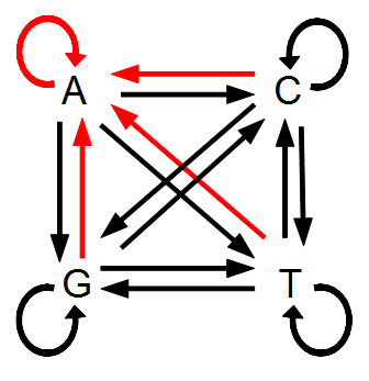
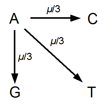
Imagine a nucleotide can mutate with the same probability to any other nucleotide, so that the mutation rates in all directions are equal and symbolized by μ.

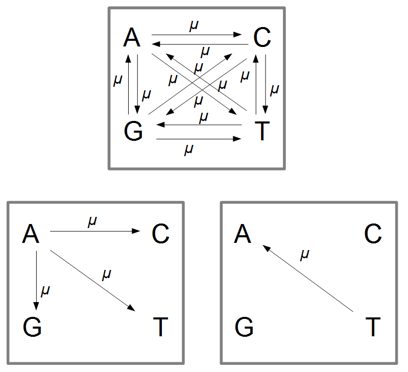
So from the point of view of the "A" state you can mutate away with a probability of 3μ (lower left above).  However, another state will only mutate to an "A" with a probability of μ (lower right above); the "T" could have just as easily mutated to a "G" or "C" instead of an "A".

When we talked about the reversible mutations one result was that the equilibrium frequency of a state was the rate of mutation to that state divided by the total rates of all mutations.  We can see above that there is one μ moving toward "A" from a specific state and 3μ moving away.  This gives 1μ/(3μ+1μ) or 1/4 as the predicted frequency of "A" in a DNA sequence at equilibrium, which makes sense, if mutations occur in all directions at equal frequencies then we expect 25% of the nucleotides to consist of "A's".  This is also true if we look at all the possible mutations simultaneously.

There are three paths to "A" and nine other paths for a total of 12.  3/12=1/4.

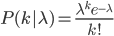
Now it's time to talk about the Poisson distribution.  This is a convenient distribution to use in many cases where the probability of an individual event is rare, events occur independently, and we are thinking about intervals of continuous time (or space).  Classic examples are the number of people in a line at the bank per hour, or the number of letters received in the mail per day, or the number of Prussian soldiers killed each year by horse kicks, or less classic, for example, the number of meteors larger than 10 meters in diameter that impact Earth's atmosphere each decade (this happens to be slightly less than one on average).

The probability of each number, , of events can be calculated given the average expected number, , according to:

So, if on average we expect events, the probability of zero, one, two, etc. events looks like this:

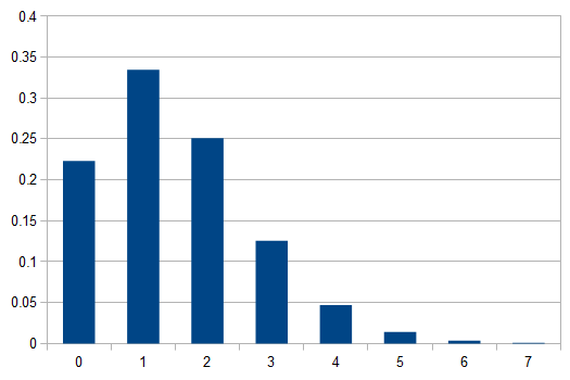
In words, the probability of no events is 22.3%, one event is 33.5%, two events is 25.1%, three events (twice the average) is 12.6%, ... seven events is less than 0.1% and the probability of eight or more events, given the average is 1.5, is practically zero.

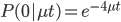
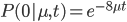
Of special interest is the probability of no events, .  Then the equation simplifies to:

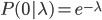
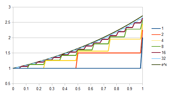
So, as the mean increases (x-axis below) the probability of zero events (y-axis) drops according to an exponential distribution.

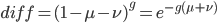
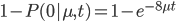
By definition, the total probability of all possible outcomes must sum to one, "something has to happen, even if it is nothing."  So the probability of one or more events (at least one event) is one minus the probability that it did not mutate, which is the probability complement of , which can be written as (the probability that there are not zero events given the expected number of events):

To bring this back to mutations, we expect some number of mutations to occur over an interval of time.  So we multiply the mutation rate, , by time, , to get an expectation. Starting at one site, there are three possible paths moving away, so there are three opportunities for mutation, so it seems that each time step the mutation rate is .

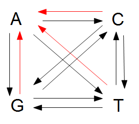
However, for mathematical convenience we are going to add a strange possibility.  It is easier to work backwards and say if the site did mutate at least once, the probability it mutated to a "G," for example, in the last step is 1/4, no matter how many total mutation steps occurred.  But this is not true under the model we drew above if the site was a "G" before mutating.  The same state can not mutate to the same state, or it wouldn't be a mutation as we understand it.  Anyway, let's allow for the time being the possibility that a site can "mutate" back to itself, also at rate μ.  So we get a visual model like this:

Now the potential for mutation each time step is .

This is the mean of the Poisson, .

Actually there is a 2X correction.  The DNA sequence is inherited from a common ancestor along each lineage to each modern species that we are comparing.  So the actual distance in twice the time to the common ancestor.  .

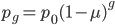
So, the probability of a DNA site not mutating between two species is

The probability of at least one mutation is:

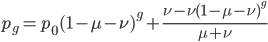
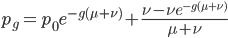
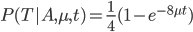
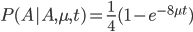
Now, in our modified model, if there has been at least one mutation, the probability you end up at a specific state like a "T" is 1/4.  Combining these we get (say we started with an "A"):

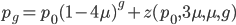
In fact, ending back at an "A" is also:

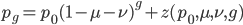
The probability that the same site is different in the two different species is:

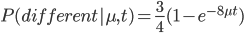
Because, with one species at one state at a site there are three possibles ways to be different in the other species, and to do this at least one mutation had to occur between them.

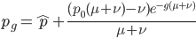
We can see the equilibrium distance from the equation.  raised to a large negative value approaches zero.  and this one is multiplied by .  So at equilibrium the distance between two sequences, that began as identical, is 75%.  In other words, just by chance 1/4 of the sites will happen to match because there are four nucleotides to choose from.

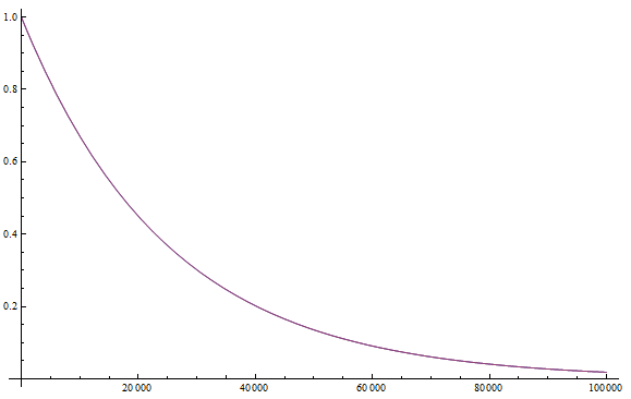
If we plug in realistic mutation rates, like we get this kind of curve.

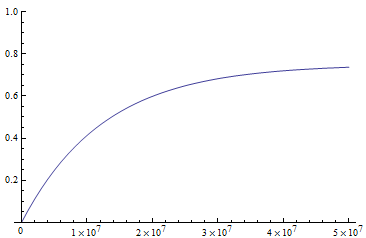
The x-axis major units are 10 million generations (or time units).  The trajectory is near equilibrium at 50 million generations.  Also, the per nucleotide mutation rate is much smaller than the per gene mutation rate where there are many more nucleotide sites that can disrupt the gene.

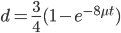
Ok, so our expected distance (), the fraction of nucleotides that are different, is

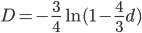
What we really want in species comparisons is a measure that is linear with time.  Let's set , which is time linear, substitute it in and solve.

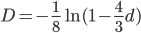
This takes the raw distance (blue curve below) and converts it (assuming the mutation model is a reasonable approximation) into a time linear distance between species (red line below).

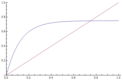
If you look up the Jukes-Cantor distance correction in other places you may see different numbers.  This is because there are different ways to scale mutation when you write down the model.

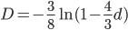
One approach is to divide all the mutation rates by three (μ/3), so that the total rate of mutation away from a state is μ.  This seems reasonable and gives

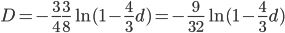
Another common variation is to ignore the X2 correction for two lineages from a common ancestor and just think of it as a single lineage from a common ancestor, which gives:

This last "3/4,4/3" version above is the most common way of writing the Jukes-Cantor model correction in the literature.  Of course 1/4 of the estimated total number of mutations are not really mutations as we normally think of them because they result in the same nucleotide state. If I were pressed I guess I would say the "best" estimate, in terms of intuitive definitions of mutations, of the actual number of mutation events that have occurred based on the difference of two sequences is 3/4 of the μ/3 rates with the X2 time correction:

.

This is an estimate of events over time, based on our model, that we would actually call mutations--I think. However, in the end it doesn't really matter how mutation and time are scaled as long as it is consistently applied between comparisons.  What we really want is a distance measure, from the fraction of differences out of the total, that is proportional to () the mutation rate and time (the slope doesn't matter so long as it is linear) rather than to try to directly estimate the actual number of mutations that have occurred over the time period:

If we also assume mutation rates are constant, this is simply time linear:

OK, that's enough for now.  Later I want to talk about how this connects back to the discrete time model for reversible mutations and look at an example of using this.

Here are some more photos of our flies from the microscope!

Above is a female that is a mutant at three genes.  First of all she has white eyes instead of the normal red wildtype.  This is a mutation at the white gene on the X-chromosome and can be written as w ^-.  She also has a darker body than normal; this is a mutation at ebony (e^-) on the third chromosome (fruit flies have four pairs of chromosomes; the X-chromosome is also called the first chromosome).  Finally, the bristles are shorter and twisted instead of long and straight.  This is easier to see in the picture below.

This is due to a mutation at another gene on the X-chromosome called singed (sn^-).  Some mutations are more subtle, but these are easy to see and score in a large number of fly offspring.  In past years the students in the genetics class lab mapped the location of genes on the chromosome by measuring rates of recombination with these visible mutants.

Below is a very young adult that has just eclosed (emerged from the pupal case).  They are very pale and shaped funny when first eclosing.  (This one also has wildtype eye color and normal long straight bristles.)

The wings have not fully extended yet and are still folded up.  Below is a close up.

Below is another young fly that is still pale.  When they are a bit older they swell up like this.  The wings are fully extended but they curl up because of a dominant mutation at a gene called Curly (with a Cy^- allele, and the fly has a Cy⁺/Cy^- genotype) on the second chromosome.

Here is a comparison to an older adult female (that does not have the Cy ^- mutant allele).

Also, there is a dark, off-center, spot on the ventral abdomen of newly emerged flies.  It is the remains of the last larval meal in the gut before becoming a pupae and is sometimes referred to as meconium for convenience (though technically this may only apply to mammalian infants).

This is what you want to look for to collect unmated females to set up new crosses.  They do not mate within the first few hours of eclosion and this appearance (pale abdomen with a meconium spot) is something fly geneticists spend a lot of time looking for.  The even younger, shriveled up, unfolded wing, stage does not last as long.