This semester I have been working through some basic population genetics background to prepare for a class I plan to teach next spring.  One place to start is on the predicted effects of mutations.  The simplest model to begin with is one of irreversible, one-way, mutations.  Imagine a functional gene sequence and that mutations can occur to disrupt the gene function, effectively turning it "off."  I like to mention working on cars for analogy.  If you made small random changes to car parts, the most likely outcome, if anything happens at all, is that you break the function of the part and render it useless (rather than gaining a new and different function or, even-rarer, improve its function).

So say the mutation rate is really high, like 10% per generation, and you start off with 100% functional gene copies.  Then after one generation only 90% of the copies are functional because of the 10% that mutated (1 - 0.1 = 0.9).  In the next generation 90% of the 90%, or 81%, are still functional; in the third generation 90% of the 90% of the 90%, or , remain functional.  (There are also mutations in the already mutated alleles but these do not change the phenotype (it is still an inactive gene function) so these are ignored and lumped together; only the mutations in the remaining unmutated alleles are kept track of.)  So it is easy to see that after generations with a mutation rate of the fraction of unmutated alleles is .  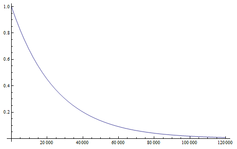Our example gives the following graph over the first 20 generations:

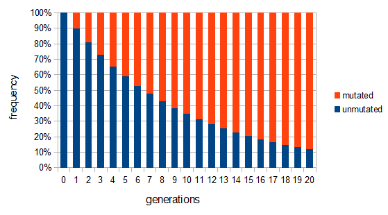
This curve follows a (discrete) geometric distribution and over long periods of time can be closely approximated by a (continuous) exponential distribution.   This is an example of exponential decay like the classic curve of radioactive decay and the idea of radioisotope half-lives.

The same type of curve and equation applies even if we do not start off at a 100% frequency of one allele.  Say the functional allele is at 50% frequency, , then one generation later 10% of the 50% mutate leaving 90% of the 50% unmutated, .  Generally, if the starting frequency at time zero is then the frequency after generations, , can be calculated as .

Another way to look at this is (the frequency at time g is equal to the frequency in the generation before, g-1, multiplied by the fraction that did not mutate, . However, 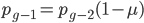and 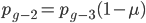, etc.  Substituting in the reverse order, 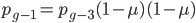and 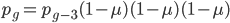, etc.  Quickly we see that from a beginning point the equation becomes because we are multiplying g-times.

---

One reader did not like the previous paragraph and found it hard to understand; I'll try to present it again here in just equation form.

, if is defined as the number of generations after exists.

---

Actual mutation rates vary widely over several orders of magnitude but in general are much lower than the example of 10% per generation I used above.  Often, the mutation rate affecting the function of a gene is on the order of to per generation.  The mutation rate at a single nucleotide site in a DNA sequence is on the order of .  It can be tricky to measure mutation rates directly.  Often mutations are recessive or are not completely visible as a phenotype.  However, in humans there have been several studies focusing on achondroplasia (a form of dwarfism) to measure mutation rates.  The mutant allele is dominant, so a single copy results in the dwarf phenotype.  The phenotype is fully penetrant (if you have the allele you have the phenotype, in contrast many human traits are incompletely penetrant).  Finally, the phenotype is unambiguous.  These factors make measuring the rate of appearance of achondroplasic individuals from birth records ideal for directly measuring mutation rates.  Results from different studies vary but rates on the order of 1 in 25,000 or have been found.

Obviously, selection and genetic drift are important factors affecting allele frequencies in real populations.  Mutations in the FGFR3 gene that result in achondroplasia are removed from a population by selection and never attain high frequencies.  However, for the moment I am keeping things simple by only looking at the predicted effects of mutation rates.  Imagine a species that moves into a cave system and then the population is cut off from the outside world (so called troglofauna, or cave animals).  If genes are no longer needed in the cave environment, like ones involved in eye development or pigmentation patterns, how long would we expect functional alleles (different forms of a gene) to remain in the population?  In other words, mutant non-functional alleles are no longer removed by selection.

Using a little algebra

can be rearranged to

by dividing by .  Then take the of both sides

and divide again to solve for the number of generations

.

Using from above and setting (so that the frequency at time is the starting frequency at time zero, we get a half life of the functional allele of 17,328 generations.

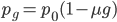
Setting we find that after 115,127 generations 99% of the population's alleles have mutated to the non-functional form.  The curve for the first 120,000 generations looks like this:

showing the initial steep drop and then leveling off of the change in frequency due to mutations.

If we consider a generation to be about a year long for many species than after about 120,000 years (which is not really that long) any genes that do not have functions that are selected for are expected to be inactivated and functionally lost from the genome.  This can easily explain the pigment-less, eyeless cave fish found in the southeastern US.

Turning this around, if a gene is found to be functional and preserved in the genome and at a high frequency (>90%) in the population, it follows that it is being maintained by selection in the recent past.  Humans along with many other primates (and independently guinea pigs) have lost the ability to synthesize vitamin C because of mutations in the GULO gene (the remnants of which still remain on our 8th chromosome). This suggests our distant ancestor had plenty of vitamin C in their diet for thousands of generations and that mutations in GULO were not removed by selection.

This also suggests a way to measure mutation rates by changes in allele frequency in the absence of selection, if we know when the selection pressure was removed.  Imagine bacteria that carry a plasmid with resistance to two different types of antibiotics.  Initially they are kept on media containing both antibiotics, but then are transferred to a plate containing only one (to maintain the plasmid).  We know that bacteria, under optimal conditions, can divide every 20 minutes or so.  We could periodically take out a sample and assay what proportion still maintain resistance to the missing antibiotic.  The equation above can be rearranged again so that the fraction resistant, and the time on the new media, can be plugged in to estimate the mutation rate.

However, this does ignore any possible fitness cost to the bacteria to maintain antibiotic resistance, and selection could also drive the inactivating mutations to high frequency in the population (this could also be occurring in cave species; an energetic cost to producing pigments, or the presence of eyes providing a source of infections, could result in selection inactivating the genes even faster than predicted by mutation).

In fact, growing bacteria continuously in a chemostat and periodically checking for mutations in resistance to infection by bacteriophages (viruses that infect bacteria) is a classical method to assay mutation rates.  Different compounds can be added to the chemostat to test if they raise or lower mutation rates.  The assumptions used in measuring these mutations rates are essentially the same as presented here in this post, with one exception.  When the mutant frequency is very low the curve is nearly linear.  So

is almost equal to

when is near 100%.  This is because almost all of the alleles are unmutated, so essentially any potential mutations that can occur do occur on unmutated copies.  In terms of the mutant frequency , if the mutation rate is 1% and at first no mutants are present, in the first generation the mutant fraction is .  In the second generation , which is almost 0.02.  In the third generation , which is almost 0.03, etc.  The low frequency approximation can be rewritten as (the mutant fraction each time step adds the same quantity to the initial number of mutants).  This is a linear equation of the form , where b is the y-intercept and m is the slope of the line.  So in this case the slope of the increase in mutant frequency is equal to the mutation rate.  If the slope increases when chemicals are added to the broth the bacteria are growing in then they are potential mutagens.

At any rate, the phenotypes of cave species and the predicted rapid inactivation of gene function by mutation in the absence of selection maintaining the function is a nice, simple, easy to understand example of inferred evolution.  The mutations that can occur in bacteria are also a nice observable example of evolution in action.

OK, that's enough for now.  In future posts I will discuss some more complicated mutation models.