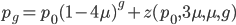
In the earlier post about a simple model of reversible mutations I used a discrete time approach. Events happened in defined time-step generations. We ended up with something that looked like this to describe the change in frequency over time measured in generations,  :
:
I will leave the details in the earlier post. However, I want to mention that  and
and  are mutation rates and I have put a
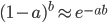
  function here to represent the part of the equation that approaches
  , the equilibrium frequency, as the number of generations, , get large. Also, we ended up with a difference in allele frequency, when starting at the extremes,
  and
and  of
of
My point being that  appears a lot.
In the Jukes-Cantor model we used a continuous time approximation to be able to use the Poisson distribution. So, for example, we had the probability of no mutations occurring along the lineage from an ancestor equal to:
 ,
,
where is again the mutation rate per unit time and the total time is  .
.
On the surface these look very different but lets change some things around.
In the Jukes-Cantor model we kept track of four different mutation rates all at a rate of . In the simple reversible model we kept track of two mutation rates at rates of and .
If we used the form of the reversible model, but used four equal mutation rates, we would have something like:
This is the frequency of the allele that either has not mutated (or has mutated back from another form, which is wrapped up in ).
Let's plot together the probability the allele has not mutated for each model:  and
and  (with a mutation rate of
  ):
):
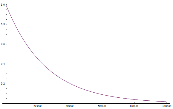
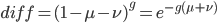
There are two curves plotted, but they are almost exactly overlaid with one another. Here is a plot of the difference in the two curves:
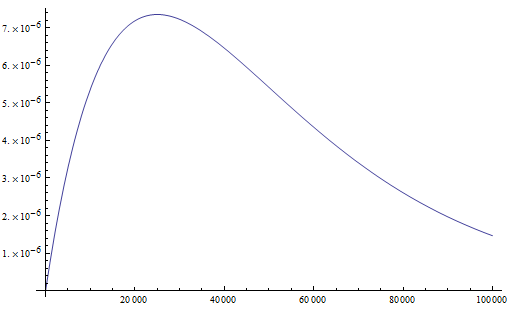
Notice the scale of the y-axis, frequency differences in the millionths. Also, as the number of generations gets very large the difference approaches zero. This indicates the difference in continuous time and discrete time assumptions, which disappears as the individual time intervals become relatively small. Also,
In fact, this is one way  can be defined as one approaches a limit from discrete time to continuous time. For example see the description of and (continuously) compounded interest. As an investment is compounded at smaller and smaller time intervals, the effect of repeatedly compounding increases the final amount but at a diminishing rate because the time to gain interest between compounding events is over smaller and smaller units of time. At the limit of continuous time with infinitely small time steps
  becomes
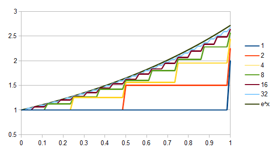
In the graph above time is on the x-axis. The initial value is compounded at the same rate but over smaller units of time (the inverse of 1, 2, 4, ...). The curve at the limit follows  .
.
The results of the earlier mutation models can be revisited knowing this.
The first model of irreversible mutations:
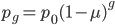
can be written in a continuous time approximation as:

And the reversible mutation model:
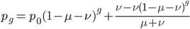
can be written as:
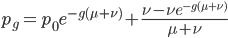
or
 ,
,
where  , the equilibrium allele frequency.
Also, the maximum difference in allele frequencies in the reversible model becomes