I have been trying to start with some basics and build these posts upon each other, so I can reference back to earlier posts for background.  However, I just found out something that interests me and wanted to share it before I forget the details so I will jump ahead a bit.  It turns out that although this is in some ways a strange example, in other ways it is easy to understand and perhaps does not need that much background.  (Although, it does build a bit on the Bernoulli distribution in my last post; the reason I went ahead and made that post first.)

I haven't really talked about genetic drift yet on this blog.  Long story short genetic drift is evolutionary sampling error.  When you take a sample from a larger population you are likely, by chance, to over- or under-represent certain categories in your sample.  The larger a sample you take the smaller this error is as a proportion out of the total.  The same things happens biologically in sampling alleles from a population to make up the next generation.  The larger the sample (the more parents there are) the smaller the error is.  In other words, generally speaking, the larger the population the less alleles change in frequency between generations.  Conversely, genetic drift and allele frequency change is accelerated in small populations (or in populations where very few individuals are reproducing).

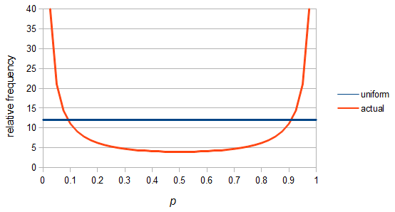
SNPs are single nucleotide polymorphisms that are found all across the genome.  In general they have two alleles, a C and a T for example.  If we genotyped a lot of SNPs across the genome what frequencies would we expect to see the alleles at?  It turns out that we do not expect to see a uniform allele frequency distribution.  There are not the same number of alleles at 10% frequency in the population as there are at 20%, 30%, etc.  Instead there is a U-shaped distribution where most alleles are at very high and low frequency (if one allele in a pair is at 5% then the alternative alleles has to be at 95% so the curve is symmetric) and fewer alleles are at intermediate frequencies.  These two types of curves are plotted below:

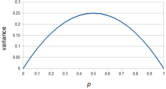
So what is the actual shape of the expected curve?  To understand that we have to first realize that allele sampling is a binomial process, either one allele or the other is sampled, this is repeated several times, and the new collection makes up the next generation.  Like the Bernoulli distribution the variance in a binomial process is greatest at the middle frequencies and is . If we normalize this on a scale of zero to one dropping for the moment this is identical to the curve for the Bernoulli variance.

When an allele is rare, it only gets a chance to be sampled a few times, and does not have much opportunity to change in frequency.  The most dramatic change is if it is lost from the population completely in the next generation and this is not really a big change because it was rare to begin with.  If alleles are at intermediate frequencies there are many chances to be sampled so the possibility of "error" at each individual sampling is magnified.

So, the change between generations is largest at intermediate frequencies.  Now imagine people migrating within the continental US.  Say that people move very little each generation on the East and West coast.  A family's children tend to live in the same city as their parents or at most move to a neighboring city.  However, on the Great Plains in the middle of the country families tend to move around a lot.  So one families children may grow up to live 100s or over a thousand miles from their parents.  Over time, with this pattern, we expect people to accumulate on the east and west coast and, over the span of several generations, to spend less time in the geographic center of the country.  This predicts the greatest population levels on the coasts and the lowest population in the middle.

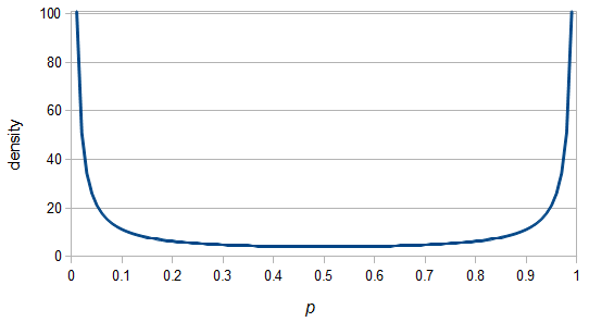
So, because of the binomial variance, we expect alleles to spend less time at intermediate frequencies where the change in frequency is greatest due to genetic drift, and spend more time at high and low frequencies where drift and variance are lower.  In fact, so long as this process is only driven by genetic drift this is the only factor that we need to consider and we expect the population of allele frequencies to be the opposite or inverse of the variance.  So the frequency of different alleles is expect to follow this distribution:

And gives the following curve:

This curve is known as the site frequency spectrum and is expected as the alleles reach a mutation-drift equilibrium.  The alleles themselves however are still drifting up and down in frequency but the ones that move away from each frequency are exactly replaced by ones moving into that frequency class so this is a steady state distribution (rather than an equilibrium distribution in the usual sense--specific alleles do not remain at a single frequency value).

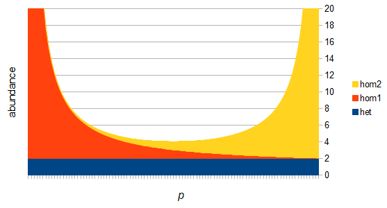
Up till now I think this is very straightforward and understandable (at least to the limit of my writing skills).  We can use this curve as-is to make some insights into the genotype distribution.  For example, according to Hardy-Weinberg heterozygotes are most common at intermediate frequencies and follow but alleles are least common at intermediate frequencies, so we can combine these to see what the distribution of heterozygous genotypes looks like in terms of actual relative numbers across loci (sites in the genome).  Interestingly these two curves cancel out when multiplied together: .  The number of heterozygous genotypes is not a function of and is uniform for all values of .  So, for example, even though there are many more homozygous genotypes than heterozygotes at low frequency, there are many more alleles in the genome at low frequency, so the actual number of heterozygous genotypes remain the same as the number seen at intermediate frequencies.

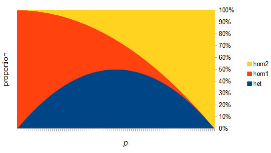
There are two graphs below, the first one shows the relative abundance of the different genotypes within the predicted site frequency spectrum; the second is the relative frequency of the genotypes to each other, which is basic Hardy-Weinberg proportions.  To generate the curves for the first homozygote the equation is , the second homozygote is

However, this site frequency spectrum curve has one interesting problem.  These kinds of distributions are usually normalized so that the area under them sums to one (100%).  This curve can not be normalized because the area under it is infinite.  In the graphs above you can see that it increases sharply at the edges of zero and one.  The curve approaches infinity as it moves toward an edge value of .  In several other cases it is possible to have a finite area under a curve of infinite length, but the area of this curve does not converge to a finite value; it approaches zero and one too slowly (the spikes on the edges are too "fat") and accumulates an infinite area.  (The integral  is an improper Riemann integral of the second kind. In fact the factors and also have improper integrals.)  This may seem like a nuisance but this difficulty can give us a little more insight into what is going on here.

In defining this curve, , to figure out what the site frequency spectrum looks like we made a critical assumption--that there are no new mutations and the distribution is only governed by drift.  We assumed the system was only affected by drift for convenience, but what we are really interested in is a mutation-drift equilibrium process.  How can there be alleles and variable sites if there are no mutations?  We could assume that mutations stopped at some point in the recent past and that we are looking at the distribution of the remaining alleles, but then the system would not be at equilibrium.  The key contradiction here is that without mutations we can not have variation remaining at equilibrium, so it is nonsensical, in a way, to talk about the site frequency spectrum in this case--except at two points, and .  Mathematics has "attempted" to resolve our contradictory assumptions by forcing this result to a ridiculous extreme that actually kind of makes sense.

The reason we can not integrate this curve is because all of the mass is infinitely close to zero and one, but can not quite be equal to zero and one, so it gets stacked up to infinity.  Even though we see a curve at intermediate frequencies the area under it is an infinitely small fraction of the total and we would never expect to actually see any alleles at these frequencies (under these model assumptions); the relative fraction of probability is infinitely close to zero, which is zero.  So this actually makes sense, we expect all the alleles to either be fixed or lost, at zero or one, at mutation-drift equilibrium when the mutation rate is zero.  The curve we see at intermediate frequencies is a sort of mathematical "ghost" that is left behind at the extreme limit of a zero mutation rate; we will never see alleles at these frequencies but, if we did, this is the curve we would expect them to follow.

This does not mean that the curve is not useful.  For all practical purposes the SNP mutation rate is quite small, so (speaking on a simplistic level) we might well expect actual allele frequencies to closely follow the "ghost" curve and for results from studying it to generally hold, such as the uniform heterozygous genotype abundance.  In reality though, with non-zero mutation rates, an allele can never be completely fixed or lost in a population of sufficient size, so the area of the curve infinitely near zero and one will be zero, which suggests the curve (under modified, more realistic assumptions) can be integrated and converges to a finite area...  but this will be the subject of another blog post.